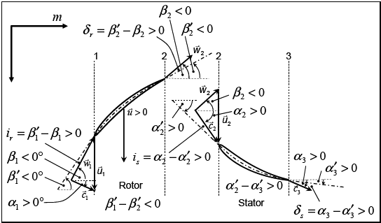
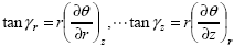
When looking along the axis of the machine in the direction of flow we have a cylindrical coordinate system (r, θ, z). The positive θ direction is the clockwise direction when viewed along the meridional direction from the inlet. The angular coordinate (theta) is taken as positive in the clockwise direction and negative in the counterclockwise direction. The normal case considered by Vista TF if the speed of rotation is specified as a positive value is clockwise rotation when looking along the axis in the direction of the flow so that the angular coordinate increases in the rotational direction. See Figure 14.4: Coordinate System used by Vista TF below.

Figure 14.4: Coordinate System used by Vista TF

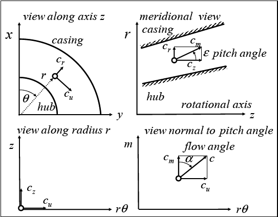
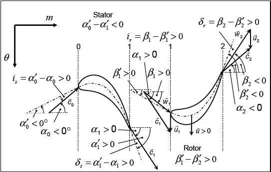
Blade angles are then defined from the axial and radial directions in a similar way using the positive theta direction as a basis. The rate of change of the angular coordinate with the meridional direction then defines the sign of the blade angle, and this applies for the blade angles, flow angles and also applies to the blade lean angles; see below. As you move along an axial rotor blade in the axial direction of a clockwise rotating machine then the blade wrap angle (theta) steadily decreases as the blade is sloped backwards against the rotational direction, and so the rotor blade angles are negative. This also applies for radial impeller outlet angles, which are generally also backswept. In fact, at the outlets of both compressor and turbine rotors, a negative blade angle is expected for a machine rotating in the clockwise direction. In stator vanes, the angular coordinate generally increases along the blade in the meridional direction so that the blade angles are generally positive.

This rule works for axial, radial, and mixed flow compressors, provided that the meridional direction is used as a basis. In a turbine stator, theta also increases positively from LE to TE and, in a turbine rotor, theta decreases from LE to TE. There are some exceptions to this rule, related to high camber at leading edges to adapt the flow to the incoming flow direction, as shown in Figure 14.5: Sign Convention for Blade Angles in Vista TF for a highly cambered turbine stator. This situation can also occur in blades with leading edge recamber in ventilator blades in channels of high curvature.

Figure 14.5: Sign Convention for Blade Angles in Vista TF

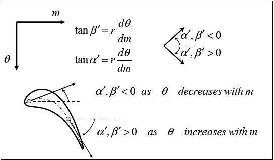
Figure 14.6: Sign Convention for Angles in Vista TF shows the angle definitions used in Vista TF; these are consistent with the blade angle definitions. The sign convention for velocity values is that an axial velocity component in the positive axial direction is positive, a radial component in the positive radial direction is positive, and a circumferential component in the positive angular direction (theta) is positive. Note that the rotational speed has an associated sign, so that clockwise rotation corresponds with positive rotational speed and counterclockwise rotation corresponds with negative rotational speed.

Figure 14.6: Sign Convention for Angles in Vista TF

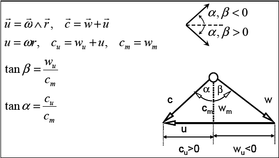
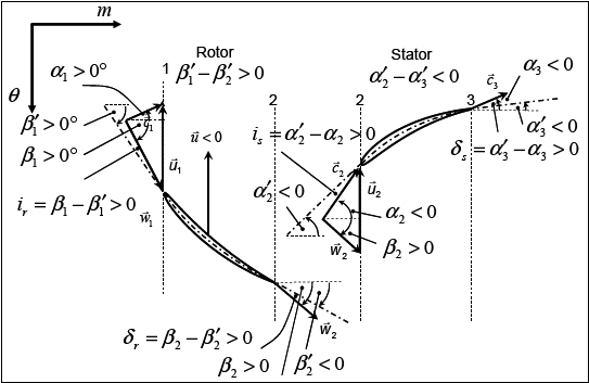
As examples of this notation, Figure 14.7: Sign Convention for Blade and Flow Angles in Vista TF for a Clockwise Turbine and Figure 14.8: Sign Convention for Blade and Flow Angles in Vista TF for a Clockwise Compressor show the velocity triangles with blade angles and flow angles for typical axial compressors and turbines rotating in the clockwise rotational sense.

Figure 14.7: Sign Convention for Blade and Flow Angles in Vista TF for a Clockwise Turbine

Figure 14.8: Sign Convention for Blade and Flow Angles in Vista TF for a Clockwise Compressor

To demonstrate that this notation can be used for counterclockwise rotation and for counter-rotating blade rows, Figure 14.9: Sign Convention for Blade and Flow Angles in Vista TF for a Counterclockwise Turbine, Figure 14.10: Sign Convention for Blade and Flow Angles in Vista TF for a Counterclockwise Compressor, and Figure 14.11: Sign Convention for Blade and Flow Angles in Vista TF for a Counter-rotating Compressor show these cases.

Figure 14.9: Sign Convention for Blade and Flow Angles in Vista TF for a Counterclockwise Turbine

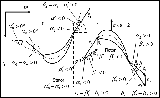
Figure 14.10: Sign Convention for Blade and Flow Angles in Vista TF for a Counterclockwise Compressor

Note that the rule given above for blade angles is applied independently of the rotational direction of the blade rows. For example, if the blade rotational speed is defined as negative then the blade angles of a compressor rotor would typically be positive as the angle theta then increases in the flow direction, as shown in Figure 14.10: Sign Convention for Blade and Flow Angles in Vista TF for a Counterclockwise Compressor.

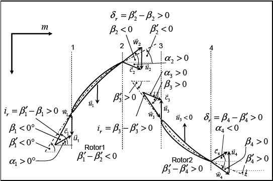
Figure 14.11: Sign Convention for Blade and Flow Angles in Vista TF for a Counter-rotating Compressor shows an example of a counter-rotating compressor with two rotors, the second rotating in the reverse direction. In this case the first rotor blade row has negative blade angles and the second rotor with reverse rotation has positive angles.

Figure 14.11: Sign Convention for Blade and Flow Angles in Vista TF for a Counter-rotating Compressor

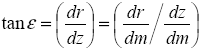
Consider a point q on a radial impeller blade camber surface, as shown in Figure 14.12: Definition of Angles. We can define the blade lean angles,   and   as the angle made by the blade fibers with a radial line and the angle made with an axial line, as follows:

In order to assist the understanding of the angles,  ,  , and ε, the analogy to the angles known as yaw, roll, and pitch of a sailing boat might be useful.

Figure 14.12: Definition of Angles

Notes on  :

Notes on  :

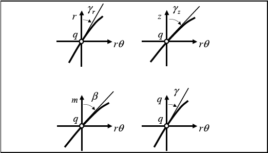
The angle   is the inclination of a meridional streamline to the axial direction:

which on the hub and casing walls becomes the meridional slope angle of the walls.

Internally the program uses the angles   and   to calculate  , which is the effective blade angle measured from the meridional direction.   is defined as:

Notes on  :

If the program fails to run at all, then this is usually a sign that some of the formatted input data is not correct (no empty lines where these were expected, or an empty line where data was expected, or similar formatting problems). The screen monitor information then says that the file has broken down in a particular input subroutine; this provides a clue for identifying which file has an incorrect format. Most straightforward errors caused by new users or new cases are related to the data input files, which are absolutely rigid with regards to the lines of data and which do not accept an empty line where a line of data should be. No built-in consistency checks of the input data are made, so errors of this nature can easily occur, especially at the beginning of a completely new calculation. To help avoid this type of error, you can copy lines from similar existing input files.

The program might report the name of the input file that contains an error. Should such errors happen, you should examine the .hst file where the input data is recorded. From this, you can determine which file has not been correctly read or might have errors, and also which part of that file has been successfully read.

If the program reads all the input files, starts successfully but then fails before the iterations begin, then this is often a problem related to the specified flow and speed conditions in the input data or the geometry specification, and these should be checked. These errors are usually related to errors in the units of the specified data (flow conditions, boundary conditions, geometry, empirical data, and so on). A typical user error of this type is that the diameter in meters is needed as a reference value for the size in the flow information (.aer), but the user specifies a radius because the coordinates in the geometry file (.geo) are radius values in meters. Another common error with users is to specify the geometry in inches rather than meters. Another typical user error of this type is that the pressure is specified in bars whereas it is expected to be in N/m². Other errors may be related to the fact that the specified flow conditions imply choked flow or reverse flow. A useful consistency check of the flow data is made where the following information is printed:

Vista TF: Axial compressor calculation
--------------------------------------
Estimated mean flow coefficient cm/u at first rotor inlet = 0.4567
Estimated mean Mach number cm/a at first rotor inlet      = 0.4426

These values may be used to determine whether the mass flow, speed, and other data, have been specified sensibly, by comparing them with typical values of these parameters for the applicable machine type.

If the program runs, but breaks down after only a few iterations, then this can often be a sign that some of the input data is still not correct because the program is generally very reliable. Here the strategy is to reduce the value of the maximum number of iterations to a lower value than that at which the flow breaks down (reduce the value of the parameter max_it_main in file .con), to rerun the case, and then to examine the results in the .hst and .out files. The errors are usually related to mistakes in the specified data (such as flow conditions, boundary conditions, geometry, and empirical data) rather than mistakes in the numerical method, and these data problems can then often be identified from un-converged results or values provided in the .hst, .txt and .out files. It can also be useful at this stage to examine the plot files of the initial geometry set up by the program, which is named test_prefix.txt or test_prefix.csv. This can often identify aspects of the geometry or flow data that are inconsistent.

If the program runs, but the results are extremely unexpected, such that a pump impeller or a compressor stator blade row has been interpreted by the program as a turbine row, then the blade angle definition should be checked. The program attempts to identify the type of blade row from the geometry specified, but in some cases the rules that have been programmed may fail. For example, a compressor stator is identified as a stator blade row which turns the absolute flow towards the meridional direction, so that the blade angle decreases from the leading edge to the trailing edge through the blade row. In some special cases, such as an axial compressor stator with a degree of reaction above 100% or rotor blades with extensive local leading edge recamber, the blade may have other blade forms. In these cases it is possible to specify additional data in the geometry file (see parameter i_row below) to overwrite the program’s own attempts at blade type identification. Geometry produced by BladeEditor contains blade type information provided that, in the blade feature within BladeEditor, a blade type (rotor or stator) is specified.

The program has several different internal convergence checks, but a converged solution can be achieved only if all of the internal loops also converge, so only one convergence criterion really needs to be checked, which is the convergence of the meridional velocity.

The most important convergence check is the maximum error of the local meridional velocity anywhere in the flow field, expressed as a percentage of the local meridional velocity and denoted as error_cm (%) on the screen and in the output files. During the iteration process, the maximum value of the change in the meridional velocity in the whole flowfield between one iteration and the next (delta_cm%) and the location of the maximum error is printed onto the screen every 10 iterations and into the history file for each iteration. The local value of this error is also printed in the output file and into the .csv and .txt plot files. To achieve convergence near machine accuracy, use a maximum value of 0.01% as a convergence criterion. Note that this corresponds with a maximum residual error of 0.0001, which is a much more stringent criterion than an RMS residual error of 0.0001, which is a criterion often used in CFD programs. The value of the local error is output for examination with plot software. For cases that have not converged, it is worthwhile to examine the location of the maximum; this might be the location of the problem.

It is important to remember, however, that numerical methods have many sources of error. In a throughflow calculation, the so-called model errors, related to the fact that the equations we are solving do not really describe the real flow particularly adequately (in this case we solve for inviscid, circumferentially-averaged mean values on widely spaced grid lines) probably outweigh all other sources of error. A solution that is converged to a maximum error in meridional velocity of 0.5% is likely no worse in terms of its agreement with reality than a solution that converges to 0.01% or lower. So calculations that converge to 0.5% can also be considered to be converged for practical engineering purposes.

The second convergence check occurs in the innermost mass-flow iteration loop where the program monitors the number of loops required to solve the continuity and radial equilibrium equations on each calculating station. The maximum value of the number of mass flow iterations and the location of the quasi-orthogonal where this occurred is also printed onto the screen and into the .hst file. You can specify the maximum number of loops for the internal mass-flow iteration loop with the max_it_mass parameter in the control file. The recommended value for this parameter is 10. Early in the run, the program usually stops the internal loops when the value of max_it_mass is reached. Later, as convergence is approached, less then 10 internal loops are generally required. A typical converged solution may require only 1 or 2 internal loops. The error in the mass flow should be tighter than that for the meridional velocity; a value of 0.001% is currently recommended.

The third convergence check occurs in iteration to a specified pressure ratio and is related to the convergence of the inlet mass flow to a final value and the convergence of the specified target pressures at the trailing edges to a fixed value. These are written onto the output file as error_p and error_mass respectively. The same limit for the mass flow convergence is used as given above and the target pressure convergence is set internally within the program to be tighter than this. Experience shows that it is important in simulations to a specified pressure ratio to ensure that tight tolerances on these parameters are given, otherwise the program modifies the target pressures on the basis of inadequately converged data and divergence may result.

In calculations with real gas equations (release 13.0 onwards) an additional convergence criterion is included related to the change in the real gas factor of the gas. The maximum error in the real gas factor is written to the .out file.

The program reaches convergence using a relaxation procedure in which the changes in meridional velocity are damped from one iteration to the next. In some cases with closely spaced calculating stations (high aspect ratio grid) it has been identified that, although the simulation converges to a relatively low level of the maximum error in the meridional velocity of 0.1% relatively quickly, it does not always continue to converge below this level of error. In these cases you have several options. Firstly, it might be sensible to accept this level of convergence and continue to optimize the geometry of the machine. In some cases, the simulation that is not perfectly converged may indicate the existence of an unwanted flow feature as a cause of the poor convergence. Such features include: anything that creates a tendency for the flow to reverse direction; an extremely high curvature in the meridional channel; a poor grid. A second approach is to make use of other models that are built-in for the damping factors within the program, by reducing the value of the streamline curvature damping factor damp_sc and the velocity level damping factor damp_vl. Several different schemes for the damping are applied. In some cases it may be helpful to reduce both the value of damp_sc and damp_vl to smaller values than the standard values of 0.25 and 0.50. All of the parameters related to the relaxation procedure are set internally by the program.

The most common failure for the program to converge is related to difficulties in the streamline curvature calculation causing divergence of the maximum error in the meridional velocity distribution. If the program identifies a trend for the results to start to diverge then it automatically decreases the damping factors to avoid divergence by causing more damping of the solution. If the errors continue to increase, then further reduction of the relaxation factors tends to freeze the unconverged iteration at the state where the problem was identified so that there is at least no unexpected exit from the program even if the simulation does not converge. Because of this feature it is not advisable simply to increase the number of iterations in the hope that the simulation will converge. A better strategy is to calculate with a large number, say 2000 iterations, and if the simulation does not converge, restart the calculation from the restart file to reset the damping factors to sensible values. This strategy often works in difficult cases.

The program's internal numerical fix of reducing the damping factors when the error diverges is reported in the history file. If this fix does not work, then the calculation of the streamline curvatures may ultimately fail, although this only occurs in simulations that have otherwise started to have serious numerical problems. The ultimate failure here tends to be an error in the subroutine pero, called from subroutine curvature, or in subroutine parabola, called from subroutine streamlines. Both are, in themselves, generally robust. Subroutine pero is a modified interpolation routine along the lines of the so-called AKIMA splines. The breakdown is related to the numerical difficulty of calculating curvatures in a flow when the streamlines are no longer smooth and the spacing of the calculating planes is small. Subroutine "parabola" attempts to fit a parabola through internal data in the program and is also robust until serious problems occur. These errors have mostly been trapped such that an error message is printed and the program exits the calculation without breaking down. This error is trapped to avoid a catastrophic breakdown, but the program stops and reports that the streamlines are too close together.

In cases where such problems occur, it is often worthwhile simply to run the simulation again from the restart file generated from an earlier unconverged simulation or with a different initial estimate of the flowfield (which is controlled through the initial value of cm_start in the control file), because starting from better initial conditions may clear the problem found in the initial calculation. In choked flows it is generally better to start with a lower value of cm_start, as this will not be choked. In some cases it may be worthwhile for you to decrease the relaxation factors (increase the damping) rather than to let the program try to do this automatically. If this does not work then again a useful strategy is to reduce the maximum number of iterations to a lower value, say 50 to 100 (parameter max_it_main in .con file), and recalculate and examine the unconverged results. It may also help to run the simulation repeatedly with such a low limit on the maximum number of iterations because each successive run tends to get to a lower value of the maximum error. If this fails then it is useful to examine the .hst and .out files and plots of the unconverged results. These files and plots can be used to identify aspects of the design that, when improved, enable convergence to be achieved.

The program also writes the values of the local error and the local choke ratio into the .txt file so it is possible to examine this and quickly locate the location where the problems are occurring. A value of unity for the choke ratio implies that the flow is choked and a value above unity indicates that the local mass flow is above the choking mass flow of the streamtube. It may be necessary to have some fundamental understanding of how the turbomachine operates in order to identify how to remove these problems. Further comments on choking are given in Choking.

The program prints an error message if it reaches a state where the maximum change in meridional velocity from one iteration to the next is more than 400% and then it closes down the calculation. This prevents a breakdown caused by dividing by zero or taking the square root of a negative number. Should this occur it is then recommended that you repeat the calculation with the maximum number of iterations set at a value lower than that where the program stopped (see the history of iterations in the output file) and then examine the results for this unconverged point. This can help you to identify the problem.

Another common failure mode for the program where it has difficulties converging is related to difficulties in calculating reverse flow in the meridional plane; such flow is not possible with the streamline curvature method. If the program observes signs that reverse flow may occur in the meridional plane, then it attempts to apply temporary fixes to enable the iterations to proceed in the hope that the problem will be cleared. One particularly important fix (that is not reported) is to avoid negative values of the meridional velocity by setting any negative values to 5% of the mid-span value. This may be used in early iterations and later no longer be needed, but if the final "converged" result contains such values, it is not really a valid solution. This can often be identified by a difficulty in convergence at a particular location in the grid. The background to this problem is a fundamental difficulty related to the physics, whereby a strongly swirling flow in an annular duct may separate at the hub or shroud, and the streamline curvature method is inherently unable to calculate such a reverse flow. This problem becomes more serious with calculations of low hub-to-tip ratio. The use of a limit on the meridional velocity on any streamline is reported in the output.

It should be mentioned that the throughflow method is not particularly suitable for choked blade rows because the mean stream surface equations average out the flow in the circumferential direction and are therefore not aware of high Mach numbers on the suction surface of blades. In addition, any shocks that may be present in turbomachinery flows are generally not oriented in the circumferential direction so are smeared out in the circumferential averaging of the flow to determine the mean stream surface. Furthermore, the basic method is inviscid and this precludes the existence of strong shocks.

Nevertheless, despite these serious limitations, an attempt has been made to model choking in the blade rows so that, in combination with correlations, the maximum flow and the additional losses related to shocks are taken into account in the overall predicted performance. In this way, the program includes aspects of choking that are compatible with the level of empiricism of typical 1D calculation methods, and may even be more successful than these because the variation of Mach number over the span is taken into account. This is useful in a program intended for design purposes because it helps choking problems to be identified at a relatively early stage in the design process, and aids the understanding of the axial and radial matching of the blade rows as the rotational speed varies.

All aspects of special calculations for choking flows are hidden. Setting the parameter i_expert = 0 causes the program to examine choking but not limit the mass flow if choking is found to occur. This is the most robust way to run the program and is recommended for beginners. Expert users can use i_expert = 1, which limits the mass flow according to various choke models. If i_expert = 3, this parameter switches off the choke calculation for cases that may otherwise be not robust.

Choking is strongly related to the throat areas between two blade rows, so any real estimate of the choking flow should make use of accurate estimates of the throat areas. In Vista TF the shortest straight-line distance between two blade rows can be specified in the geometry file for each of the input sections, and if the values are not specified (that is, a value of zero is given) then Vista TF makes its own crude estimate of the throat areas based on its limited knowledge of the blade geometry. This estimate is, at the moment, too crude to be used accurately in the calculation of choked blade rows, and may lead to a value for the choked mass flow that is incorrect. It may be worthwhile, in some situations, to run Vista TF with no values specified for the throat and then examine the program´s own estimate of the throat areas, which are in the output file, and then run with slightly larger or smaller values specified in the geometry file, depending on the real throat areas or the choking mass flow if the latter is known.

One method that tends to work in the most difficult cases is to remove any calculating planes in the neighborhood of the throat, as suggested by Denton (1978). For turbines, no planes should be present downstream of the throat, and for compressors, no planes should be upstream of the throat. Local details of the flow calculation are lost, but the calculation can then be made to converge up to the limiting mass flow.

The key issue remaining to be solved appears to be the fact that the location of the throat is not properly taken into account, which in fact may be a fundamental limitation of a throughflow method because the throat is smeared across several planes. In the current model, it is assumed to be the leading edge plane in a compressor or the trailing edge plane in a turbine. The limit on the meridional velocity applied at the leading edge plane successfully stops additional flow from entering the choked streamtubes of the compressor, but downstream planes can still breakdown if the flow accelerates downstream of the leading edge. In turbines, no limit on the meridional velocity is applied at the trailing edge because this would otherwise cause the supersonic expansion to not take place, so that the mass flow in certain streamtubes can rise to be above the theoretically possible maximum mass flow at some calculating planes near the throat upstream of the trailing edge.

When you specify a mass flow rate, you must ensure that it is not greater than the choking value. The program may generate warning messages if the specified mass flow rate exceeds the choking value.

The output parameter choke_ratio is the ratio of the local mass flux to the maximum possible at that location. A value above unity is not a realistic solution but if the choke parameter i_expert is set to zero then such solutions can be generated. This option is available because the program is sometimes more robust under this operating mode than when i_choke is set to 1 and the full choking models are used. Note that in some multistage computations the actual specified mass flow may be below that required to actually choke the machine, but during the iterations, individual blade rows may still become choked. The program becomes less robust as choking is approached.

In some high-speed situations where it is difficult to obtain convergence with a specified mass flow, the restart file can be used to store results for a converged operating point at a lower speed and lower flow, and then the required operating condition can be obtained by starting from the restart file with new flow conditions slowly stepping to the required operating point. In a similar way, it is advisable to first set up a simulation close to the design flow, before attempting to move towards a higher flow with a higher risk of choking.

You can run a simulation with a specified pressure ratio. For a choked blade row, the shift to a specified pressure ratio is a more physical approach than specifying the mass flow because, in this case, the solution is indeterminate. In turbines with steep characteristics (little variation in mass flow with pressure ratio) this is reliable. In compressors with flat operating characteristics (large variation in mass flow with pressure ratio) this approach may be more unstable so it is not recommended for calculations close to the expected surge line.

Iteration to a defined pressure ratio makes use of the so-called "target pressure" ratio method of Denton (1978). This requires the program to make a first guess of the pressure at each trailing edge of the machine. The algorithm currently incorporated makes a crude estimate of this but it has been found that this may not be sufficient to secure convergence, especially for compressors. For this reason, you have the option to define the first guess of the pressure at each trailing edge (set i_flow = 6 instead of i_flow = 5). Even when using this option, the iteration to pressure ratio for multistage compressors is still very sensitive, and convergence is not guaranteed. If iteration to pressure ratio is used for choked blade rows, then an accurate estimate of the throat widths needs to be provided in the geometry file and the value of i_expert should be set to 1 so that the limits to the mass flow at choke are imposed. If the throat area feature is calculated by BladeEditor then the throat widths will be calculated and added to the geometry file.

As in most numerical methods, a finer grid leading to a closer spacing of the quasi-orthogonal lines and streamlines will lead to a higher numerical accuracy of the simulation. Closer spacing of the quasi-orthogonal lines for streamline curvature calculations can, however, cause instabilities in the convergence process. This can be overcome by increasing the numerical damping (lowering the relaxation factors) but this causes an increase in computational time, so a compromise is generally needed.

An aspect of the grid that affects robustness is the location of the inlet and outlet boundaries of the domain. If possible, these should be placed in regions with low flow gradients because the program has to calculate flow gradients from within the domain on the inlet and outlet planes, and it is best if these gradients are low on the boundaries. In addition, there should be at least two q-o planes upstream of the first blade row and downstream of the last blade row. This is particularly important in calculating strongly swirling flow downstream of turbine blade rows.

The relationship between the needed relaxation factors and the aspect ratio of the computational grid in a throughflow calculation was theoretically derived in a classical paper by Wilkinson in 1970 (see Streamline Curvature Throughflow Theory). His studies showed that close spacing of the quasi-orthogonal lines required more damping. The problem is related to the fact that if the calculating stations are closer together then a small displacement of a streamline can lead to a large curvature. In this case it is only possible to take a small part of the new solution forward in each iteration and so the number of iterations increases. Wilkinson derived an equation of the following form to calculate the optimum relaxation factor for a certain grid aspect ratio:

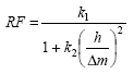
He also showed that the value given here as k₂ is actually a function of the Mach number, the flow angle, and of the method used to calculate the curvature of the streamlines. The aspect ratio of the grid () in this equation is the ratio of the calculating station length to the meridional spacing of the grid lines. The equation above was used in older versions of Vista TF to determine the streamline curvature relaxation factor with the numerical values of k₁ = 0.5 and k₂ = 20/96. The value of used was based on the largest aspect ratio that can be found in the domain. This is then further reduced if the calculations show any tendency to diverge during the iterations. The largest aspect ratio in the whole grid was used, whereby the meridional spacing is the shortest meridional distance between two adjacent grid lines, which may be on the hub or casing.

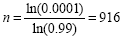
A value of 0.01 for this relaxation factor corresponds to an aspect ratio of around 15 and will lead to long calculation times because only 1% of the new solution can be taken into account and 99% is carried forward from the earlier solution. In order to reduce an error in the initial solution to 0.01% of its initial value then the number of iterations required would be

A value of 0.001 for this relaxation factor (aspect ratio near to 50) would lead to ten times as many iterations. Values of the aspect ratio larger than 15 are therefore not recommended but in cases where this is unavoidable (such as low aspect ratio blades with high span and small chord with internal calculating stations) then the program still converges but at a much slower rate.

A different stability scheme has been incorporated in Vista TF. In this, the relaxation factor ratio is calculated as:

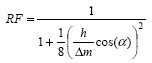
Where is the absolute flow angle in ducts and stator rows and the relative flow angle in rotor rows. In the new scheme, the relaxation factor can vary from quasi-orthogonal to quasi-orthogonal so that regions of the grid with small aspect ratios are not penalized by a locally poor grid spacing elsewhere. In addition to this improvement, experience with many difficult cases has been incorporated in the selection of the maximum relaxation factor. With this new model, you should not need to adjust the damping factors because the program does this automatically.

The new damping factor has proven to be very successful except when it is used for highly-staggered blade rows such as low flow coefficient compressor impellers or pumps. A further refinement has been added for these cases, in which the damping factor is applied to both the changes in the meridional velocity and the shift in the streamlines.

All flow gradients in the radial equilibrium equation and the curvature of the streamlines in the solution are determined by a piecewise parabolic interpolation through three points. This is a very rapid numerical procedure but experience shows that this can cause errors in the estimation of the curvature of the hub and casing if the quasi-orthogonal spacing is too wide. For the case of an axial to radial bend with circular arc meridional wall contours the error in curvature is of the order 2.5% on a grid with 7 quasi-orthogonal lines (a quasi-orthogonal placed every 15° around the bend). This decreases to 0.2% for 19 quasi-orthogonals (a quasi-orthogonal every 5°). This suggests that typical radial impellers with an axial inducer should be calculated with around 15 quasi-orthogonals in the bladed region. Moreover, the basic assumptions of the meridional throughflow method (for example: no frictional forces, axisymmetric flow, no spanwise mixing) certainly cause larger errors than this error in the curvature estimate.

It should be noted that decreasing the convergence tolerance to low values does not eradicate this error, so that for typical engineering applications a tolerance of 0.1% on cm is generally adequate because the curvature calculation is not more accurate than this. A lower value is however generally used because this confirms that numerical convergence has really happened.

Using 17 streamlines across the span is recommended. The use of such a large number of streamlines across the span brings little improvement in the accuracy when compared with experimental data compared to using only 9, but nevertheless clearly leads to fewer numerical errors in the integration of the radial equilibrium equation. 17 and 9 streamlines have the advantage that the streamlines split the flow uniformly into 16 or 8 streamtubes, providing streamlines at 0%, 25%, 50%, 75%, and 100% of the mass flow.

The limitations mentioned above on the calculation of flow gradients and curvature also determine the extent to which details of steps in the wall geometry can be taken into account. Steps, kinks and wells in the meridional contour need to be omitted because these features are typically of a sub-grid size. Generally attempts to improve the accuracy by using finer grids with more details are not made in streamline curvature calculations because this is counterproductive. These details need to be examined in CFD.

In axial turbomachinery calculations with quasi-orthogonals at the leading edge and trailing edge planes only and with flare on the hub and casing walls in the blade row followed or preceded by annular channels, inaccuracies will arise because the kinks in the contours cannot be accurately modeled.

Computing a new solution from the restart file of an existing solution, even when no changes have been made in the input data, may require 50 or more iterations to re-converge to the solution on the restart file. This effect is due to the fact that the restart file stores only a small part of the information related to the original solution, and many fine details of the solution have to be recalculated.

In running the program from a cold start (without a restart file) it is useful to think carefully about the initial value of cm_start that is specified for the control file. This determines the meridional velocity level of the initial solution and it has been experienced that an initial value too far from reality may cause the solution to breakdown. The value that should be specified for cm_start is the flow coefficient (cm/u) of the machine concerned, whereby the reference velocity used is the velocity determined by the reference diameter and reference speed (ref_d and ref_n). In flows with a risk of choking, it is better to use a low value of cm_start to ensure that the initial conditions are not close to choke. When a converged solution is available as a restart file, it should be used because, although it does not necessarily reduce the number of iterations needed, it does make the solution process more robust.

The restart file is continually updated by each converged computation, but also if the solution reaches the limit of the maximum number of iterations without converging. In a case where the solution is actually diverging, the non-converged restart file might be a worse starting condition than the program´s own initial guess, so it can be useful to discard this and start again. If a converged solution has been reached then it is sometimes useful to store the converged restart file for a better starting solution if something later goes wrong during calculations at other operating points.

As with all numerical methods, the use of unconverged results for design decisions is extremely dangerous and is not recommended. Nevertheless, examination of unconverged results can often be extremely useful for identifying numerical issues. In some cases examination of unconverged results may indicate features of the design that can be changed to avoid such problems by modification of the geometry.

One measure that has been incorporated and which may be useful during debugging of a poor calculation is to set the parameter grad_ree equal to zero. This overrides the radial equilibrium equation and leads to a spanwise constant meridional velocity (see below). This can be useful in identifying errors where flow data is inconsistent with the geometry being calculated. Another alternative that can be used with turbines is to specify a near-zero swirl velocity on the mid-streamline at the outlet of the last rotor and let the program determine the mass flow and pressure ratio consistent with this ("iteration to outlet swirl"). This has unfortunately not been thoroughly tested on enough cases to guarantee that it will always work.

If all else fails then set i_ree = 3 in the control file. Under these circumstances the value specified as grad_ree in the control file is then used to reduce the meridional velocity gradient as follows:

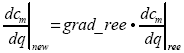
This can be extremely useful for debugging, because it can allow the program to avoid failing due to high spanwise velocity gradients. In this way, it effectively becomes a mean-line program with no spanwise variation in meridional velocity (if grad_ree = 0.0). Other parameters such as the blade speed still vary across the span, so it is not exactly a mean-line program. Most cases converge under these conditions and this ensures that the axial matching along the mean streamline of the blade rows is approximately correct. When converged it may be possible to approach a solution with the correct radial distributions by slowly relaxing the value of grad_ree towards unity. During this process, the features of the velocity gradients that cause trouble slowly become part of the calculation and this can then help to identify the problem.

Cases that do not converge well are usually either poor designs, or are good designs operating a long way from their design point. Non-convergence generally means that the design is a long way from satisfying the condition of radial equilibrium. If the flow solution converges well then this usually means that the flow is automatically close to radial equilibrium and this will generally indicate a higher-quality machine.

Considerable effort has been made to ensure that the real gas implementation is as robust as other aspects of the program. Nevertheless, errors in the definition data for the real gas can cause stability problems, because they may lead to unrealistic values of the gas properties. In some cases it may be worthwhile to run a particular case using gas equations with a real gas factor (with an estimated ratio of specific heats, an estimated specific heat at constant pressure, and an estimated real gas factor). The restart file for a converged simulation of this type can then be used for subsequent calculations with real gas properties.