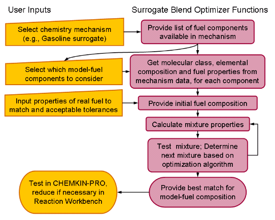
The Surrogate Blend Optimizer (SBO) is designed to allow users to optimize the
composition (blend) of a model fuel in order to match specified properties of a real
(gasoline or diesel) fuel. The SBO depends on use of Ansys Chemkin mechanism files that
include species for the fuel components of interest, with embedded tags containing
fuel properties and other identifying information for the fuel species. The
Surrogate Blend Optimizer is run from the Reaction Workbench interface, accessed by
using the Reaction Workbench icon  . The interface provides a series of panels to guide you through
the tasks in Figure 2.13: Workflow for Surrogate Blend Optimizer
.
Once a Surrogate Blend Optimizer (SBO) project is selected, an initial panel is displayed as the Operation Setup tab, as shown in Figure 2.14: Initial Operation Setup tab of the Surrogate Blend Optimizer . When a Surrogate Optimization project is started, the first step is to identify the working directory and the chemistry set (containing fuel tags) that will be used. The working directory is where the output of the chemistry processing step is stored.
After the project selection, the next option is to choose a chemistry set that contains the fuel-component species and their property tags. A tagged chemistry set that includes many common surrogate components is provided in the System Data directory, called SBO_fuel_data.cks. This tagged chemistry set provides the necessary information to estimate the fuel properties of a blend of any of the fuel components.
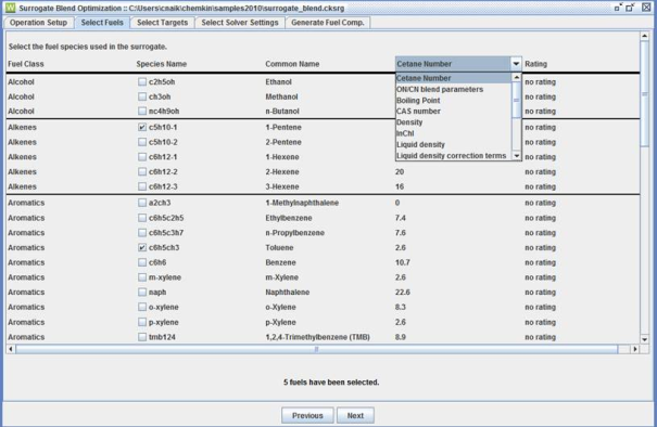
Once the working directory and chemistry set have been selected, click the Next button to go to the tab containing the list of available fuel species found in the selected chemistry set, as shown in Figure 2.15: Selecting Fuel from a chemistry set .
From the list of available fuel components, select at least one fuel component for each fuel class for which a class-composition target will be specified and any components that you think will be necessary to meet other targets. To assist in selecting appropriate fuel components, you can use the pull-down menu in the upper right of this panel to display selected properties of all of the candidate fuels, as shown in Figure 2.15: Selecting Fuel from a chemistry set .
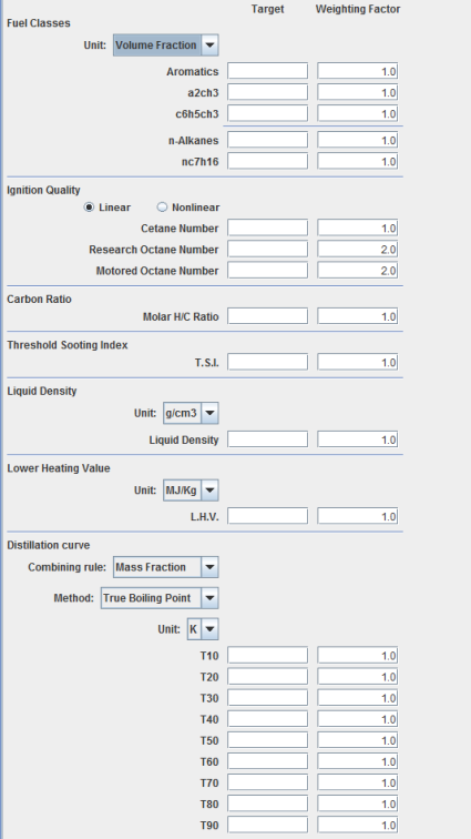
Pressing the Next button causes any selected fuel species to be added as possible components in a fuel blend matching user-specified targets. The next step is to specify those targets.
Figure 2.16: Specifying targets shows the panel used to specify the fuel property targets. Calculation or estimation methods are provided for the blending rules for the fuel properties of Research Octane Number, Motor Octane Number, Cetane Number, H/C ratio, O/C ratio, Lower Heating Value, Liquid Density, Threshold Sooting Index, and nine points on the distillation curve which can be generated by using the True Boiling Point formalism or a series of Staged Vapor-Liquid Equilibrium calculations. The points on the distillation curve are indicated by T10, T20, T30, etc., where the number indicates the percentage of total fuel evaporated at that temperature. For example, T10 indicates the temperature at which 10% of fuel evaporates. Only the properties where a target value is entered will be included in the optimization. Enter a numerical value for each target that you want met during the optimization process. It is possible to weight one target more than another, by increasing the weight to the right of the target value to a value greater than the default of 1.0. A smaller weight value indicates less importance. For example, if your most important target is to match the cetane number, you can make that weight 10.0 instead of 1.0. Weight values have no physical significance; they are only significant in relation to each other, such that weighting everything 10 would have the same effect as weighting everything 1.0.
When selecting ignition-quality indicators (cetane number or octane number) as targets, you have the choice of using linear or non-linear blending rules. The linear blending simply adds the properties together weighted by the component fraction. The nonlinear option is a more accurate method that accounts for nonlinear blending effects between certain types of components. The nonlinear option, however, requires that the non-linear blending coefficients are provided with the property data for all selected components. These are described in more detail in Non-linear Blend Parameters .
For fuel classes and fuel species, the targets can be specified in mole fractions, mass fractions, or in liquid volume fractions. When volume fractions are specified as targets for some species, the SBO finds optimum liquid fractions for other components that can best satisfy the given targets. True boiling points of a mixture are defined as temperatures at which given fractions of the fuel have evaporated. These fractions can be specified as percentages in terms of either mass or volume. The staged equilibrium calculation uses only liquid volume fraction as the defining percentage.
Note: Selecting the units for fuel composition, whether or not composition targets are entered, also determines the units for exported surrogate-blend data, after the optimization is complete.
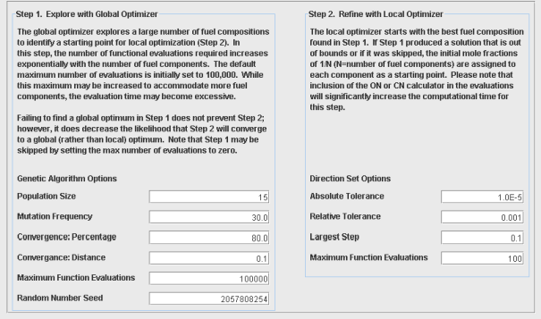
Once the targeted physical properties of the fuel are specified, then the next step is the specification of solver controls, shown in Figure 2.17: Select Solver Settings tab, with the default values . In general, default parameters on this panel should be sufficient for most optimizations. Options include parameters that alter the accuracy of both the Genetic algorithm and the Direction Set algorithm. Higher accuracy in the Genetic algorithm involves increasing the maximum iterations and sample size, and decreasing the convergence distance and percentage distance. Higher accuracy in the Direction Set involves increasing the maximum iterations, and decreasing the largest step, absolute tolerance, and relative tolerance.
Weighting factors can also be used to increase the importance of one property in relation to another. The Random Number Seed is used by the Genetic algorithm and changing its value will typically cause the Genetic algorithm to take a different convergence path, and result in a slightly different final solution. You should only change the Random Number Seed value if you wish to check that the global optimum has been found.
Note: Selecting higher accuracy options will require more computing resources.
Altering the parameters on the Genetic algorithm will affect the ability to locate the global minimum, and the altering the Direction Set will alter the accuracy of the final solution. These alterations may make finding a reasonable surrogate solution easier to achieve. For optimization problems with a large number of fuel components, the Direction Set method will find a local minimum in cases where the Genetic algorithm may exceed its limits and fail.
The last step is to run the optimization, and determine the fuel composition. Click the Next button to advance to the next tab and then the Run button to initialize the optimization. Interim results are displayed in this panel and the process can be interrupted using the Interrupt button at any time after the run is initialized.
Figure 2.18: The Generate Fuel Composition panel’s fuel composition and property evaluations of the optimized solution.
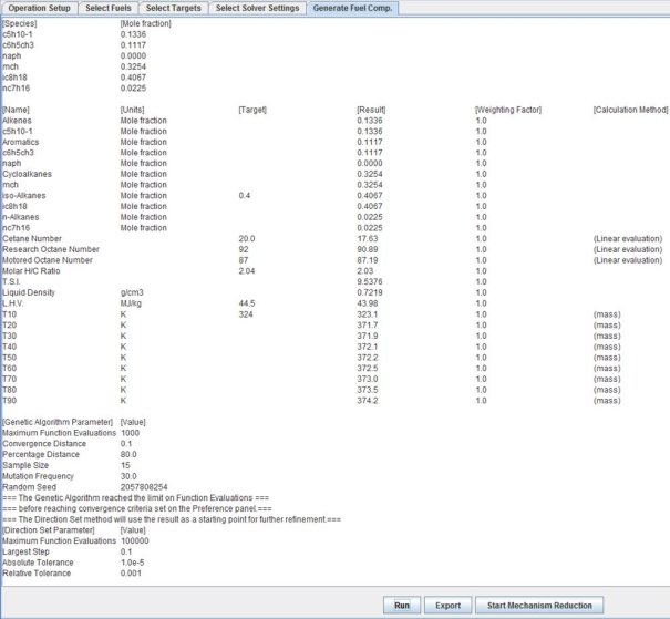
After the optimization routine finishes, the resulting fuel composition and physical properties are displayed in the output window. Exporting this information will place the species composition into a standard csv format that can then be used to initialize a composition in an Ansys Chemkin application. Note that the units of the composition exported are determined by the setup in the target-selection panel (see Figure 2.16: Specifying targets ).


