


Random fields are models that help to find a parametrization for arbitrary data on spatial domains. Typically, these are in:
1D: Signal variations (such as time, frequency, and load-displacement curves)
2D: Matrix or performance map variations
3D: Spatial variations
Random fields can be used as inputs or response to:
Find automatically a parameter that describes field variations based on measurements or simulation results
Generate random designs (such a random signals representing the distribution of temperature profiles in time, uncertain load-displacement curves, and random geometries reflecting manufacturing tolerances)
Predict field responses (meta models for signals and 3D fields)
Perform sensitivity analysis of distributed quantities (signals and 3D fields)
Perform statistical smoothening
Perform data reconstruction
oSP3D provides a variety of random field models with different properties and application ranges:
| Model Type | Inputs | Properties | Application |
|---|---|---|---|
| Empirical random field | Many measurements | Accurate description of reality | Robustness analysis, Quality control, Maintenance |
| Synthetic random field model | Few measurements | Mean + standard deviation from measurements, spatial correlation from assumption | Robustness analysis: Predict Pf based on true magnitude of variations |
| Free-form model | Few measurements | Mean + standard deviation from measurements | Needs more parameters but can localize effects on structure |
| Synthetic random field model | Single/no measurement | Artificial, global | Check if variation has impact |
| Free-form model | No measurement | Artificial, local | Sensitivity analysis with respect to input region |
Example
- Objective
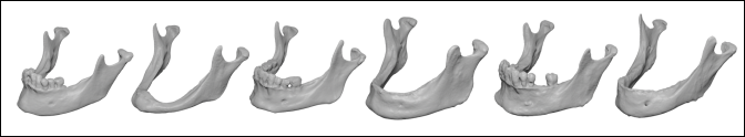
Train a random field model based on 60 measured geometries of mandibles
- Challenges
Fine meshes and large deflections
- Solution
Delete teeth from model to simplify the geometric variation pattern
The geometries were prepared using Blender scripting to have the same mesh topology. oSP3D then compared the x, y, and z coordinates of the surface nodes using a cross-correlated empirical random field model for the x, y, and z coordinates.
The result is a representation of variation patterns by a very small number of parameters. The mesh morphing is supported by mesh stabilization algorithms that reduce the amount of element distortion when applying local deformation vectors. The following images are used with permission from UK Aachen. For more information, see S. Raith, WOST 2015.
This first image shows scans of mandibles as inputs (STL):
This next image shows variation patterns (scatter shapes) and random field schematics. The left side are the identified variation patterns of a DOE of curves. On the right side are simple FEM solutions distributed on a mesh.
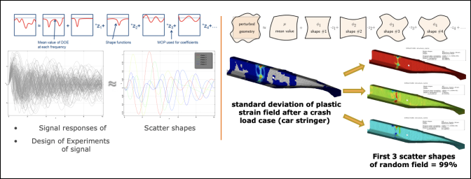
These variation patterns can be combined with sub-space parameters in a linear combination to represent either the original data (in a compressed sub-space) or to generate new field data with a correlation structure based on the training data set. This is known as the Karhunen-Loeve expansion.
By using random fields, you can use field data as inputs. The random field model translates the field into scalar parameters that can serve as inputs to other algorithms, such as meta models.