


When dealing with measurements or noisy simulation results, you often face situations where sensor data creates noise. Obviously, you do not want to use the noise as input for training a field-MOP or random field model. This tutorial shows how to use RPCA to filter noise from measurements.
RPCA is a filter for postprocessing field data before doing a statistical analysis or creating a ROM. This filter can identify noise that typically appears at random positions. In this case, you can deduce the true value from the noisy data point based on the spatial correlations from the other designs that are not noisy.
The small example for this tutorial demonstrates the power of the approach and the kind of data that can be filtered. The example creates a rectangular pixel mesh (regular grid in 2D). You assign data that is defined by a linear interpolation between the left and the right edges, whereby the actual value at the left and right edges are chosen randomly. You then assign some "sensor noise" for each design by choosing a random number of data points to be subject to noise and adding some random value to the true data points.
The following oSP3D script creates the mesh and the data. After starting oSP3D, paste this script into the command line of the Execute script window and press the Enter key to execute it.
-- Create a pixel mesh within 0<=x<=20 and 0<=y<=10 with resolution 200*100
meta = sos.createSimpleStructuredGrid(200,0,20,  100,0,10);
sos.setReferenceMesh(sos.database(), meta)

-- turn off command logging to improve make the execution of for-loops faster
sos.useCommandLogFile(false);

-- create 100 designs
for i=1,100 do
    local d = "" .. i               -- design ident as string
    local a = math.random()*100     -- left value (0..200)
    local b = math.random()*100     -- right value (0..200)
    -- create a data vector:
    local vec = tmath.Matrix(sos.numNodes(sos.database()),1)
    for k=0,200-1 do                -- loop over all data points along x axis
        for l=0,100-1 do            -- loop over all data points along y axis
            vec[ k*100 + l ] = (k/200)*a + (1-k/200)*b  -- set the field value
        end
    end
    -- create a field data object and insert data to database:
    local o = sos.createNodeDataObject(sos.database(), vec)
    sos.database():nodeDataRef():insert( sos.DataObjectKey(d, "orig"), o)

    -- now apply random noise:
    local n=math.random(1,100*200 / 20) -- get number of noisy pixels
    for k=1,n do                        -- for each noisy data point do:
        local idx = math.random(0,sos.numNodes(sos.database())-1) -- random position
        vec[idx] = (0.5-math.random())*1000 -- random value between -500 and +500
    end
    -- insert the noisy data to database
    local o = sos.createNodeDataObject(sos.database(), vec)
    sos.database():nodeDataRef():insert( sos.DataObjectKey(d, "noisy"), o)
end
Now, to use RPCA to filter the data:
In the data table, select noisy in the Field quantities list.
Select > > .
Keep the default RPCA settings:
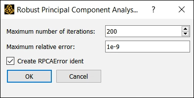
Click to start the iterative RPCA algorithm.
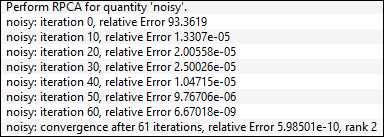
In the Log messages window, you can see the iteration history.
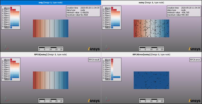
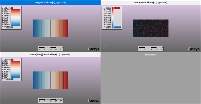
To understand what RPCA is doing, compare the filtered and unfiltered results for a selected design in the following image. The top left shows the original data, and the top right shows the noisy data. The bottom shows the filtered designs of the RPCA. RPCA can identify the random noise and separate it from the data, thereby restoring the noisy data nearly perfectly to the original data so that it can be used for further analysis.
To show the effect on field data models, create a random field model:
From the Field quantities list in the data table, select orig, noisy, and RPCA[noisy], which are respectively the original data, the noisy data, and the filtered data.
Select > > .
This example uses the default options to compute the variation shapes for all selected quantities:
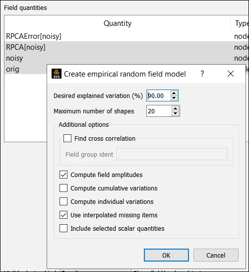
Click .
When comparing the variability fractions of the identified random field scatter shapes, you can see that the filtered quantity has the same properties as the original one.
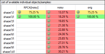
You can validate this by comparing the first variation shape. Without filtering, the random field contains the noise and takes it as "true" input data that must be represented by the model. Thus, you need many more shapes and obtain noisy variation patterns.
To examine the filtered data further, you should compare the mean value, the standard deviation, and the lower and upper value bounds.
Particularly when dealing with measurements in digital twin applications, you can use RPCA to help filter sensor errors and improve the quality of the input data, which can be signal data or geometric measurements. If certain sharp features are visible only in individual designs, RPA can remove them.