


VM-LSDYNA-SOLVE-006
VM-LSDYNA-SOLVE-006
Applied Force on Changing Element Mass
Overview
| Reference: | Any solid mechanics textbook |
| Analysis Type(s): | Added Mass |
| Element Type(s): | Solid, Shell, Mass |
| Input Files: | Link to Input Files Download Page |
Test Case
Cubes 1 to12 have edge length of 10 m and mass of 0.7 kg. Each cube has an applied load of 2000 N on one face. Cubes 6, 7, 8, 10, 11, and 12 have an additional mass that dissipates linearly from 0.7 kg to 0 kg from ti = 0 s until time tf = 0.05 s, respectively. Find the z-acceleration of each cube at ti = 0 s and at tf = 0.055 s.
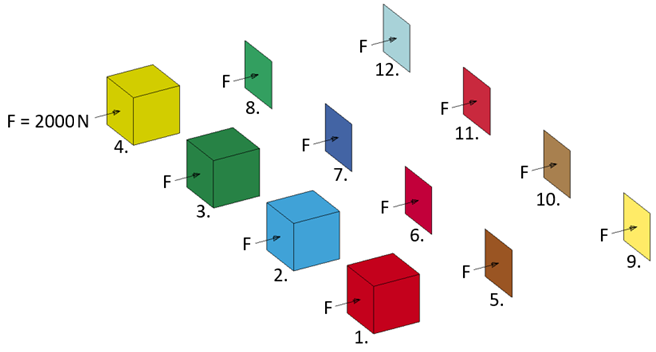
| Material Properties | Geometric Properties | Loading |
|---|---|---|
| mass = 0.7 kg | Ledge = 10.0 m | F = 2000 N |
| Added mass = 0.7 kg – 0 kg | — | — |
Analysis Assumptions and Modeling Notes
Parts 1 through 4 are solid hex elements with ELFORM 1. Parts 5 through 12 are shell elements with ELFORM 2. Shell elements have thickness 10 m. Each part is geometrically the same, but solid parts have eight nodes, while shell parts have just four nodes. Each part shares equal material properties with density 0.0007 kg/m3.
A constant pressure of 20 Pa is applied in the z-direction to a face of each part using *LOAD_SEGMENT. The pressure load is equivalent to a 2000 N force on each segment.
A combined total of 0.7 kg of added mass is distributed across the nodes of shell part 6 using ADDMASS in *ELEMENT_MASS_PART. 1.4 kg of added mass is dispersed across eight nodes of shell parts 8 and 12 using ADDMASS in *ELEMENT_MASS_PART_SET.
The final translation mass of shell part 10 was set to 1.4 kg using FINMASS in *ELEMENT_MASS_PART. The final translational mass of shell parts 8 and 12 was set to a combined 2.8 kg using FINMASS in *ELEMENT_MASS_PART_SET.
The added translational mass of parts due to *ELEMENT_MASS_PART was scaled according to a load curve. At time zero the curve starts at unity. Added translational mass is scaled down linearly until 0.05 s, at which no additional mass is added to parts.
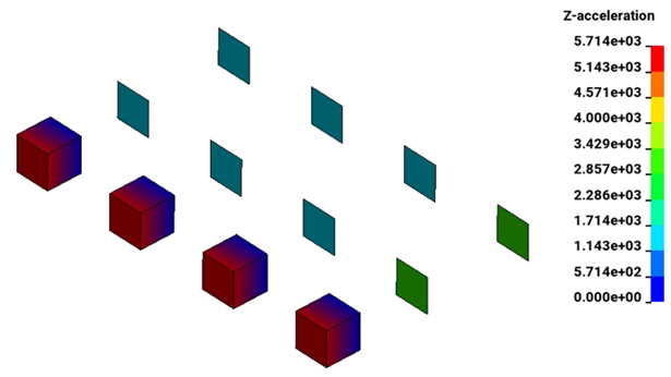
The acceleration of cubes is calculated using the equation below:

At t = 0 s, the analytical solution of az for parts 1, 2, 3, 4, 5, and 9 is 2857.14 m/s2. The acceleration az of parts 6, 7, 8, 10, 11, and 12 is 1428.52 m/s2.
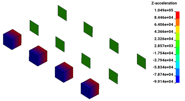
At t = 0.055 s, the analytical solution of az for all parts 1-12 is 2857.14 m/s2.
The fringe plot of z-acceleration m/s2 in the model is shown below at t = 0 s and t = 0.055 s, respectively.
Results Comparison
| Result | Target | LS-DYNA | Error (%) |
|---|---|---|---|
|
Part 1 z-acceleration, az, at t = 0 and t = 0.055 s | 2857 m/s2 | 2857 m/s2 | 0.0% |
| 2857 m/s2 | 2857 m/s2 | 0.0% | |
|
Part 2 z-acceleration, az, at t = 0 and t = 0.055 s | 2857 m/s2 | 2857 m/s2 | 0.0% |
| 2857 m/s2 | 2857 m/s2 | 0.0% | |
|
Part 3 z-acceleration, az, at t = 0 and t = 0.055 s | 2857 m/s2 | 2857 m/s2 | 0.0% |
| 2857 m/s2 | 2857 m/s2 | 0.0% | |
|
Part 4 z-acceleration, az, at t = 0 and t = 0.055 s | 2857 m/s2 | 2857 m/s2 | 0.0% |
| 2857 m/s2 | 2857 m/s2 | 0.0% | |
|
Part 5 z-acceleration, az, at t = 0 and t = 0.055 s | 2857 m/s2 | 2857 m/s2 | 0.0% |
| 2857 m/s2 | 2857 m/s2 | 0.0% | |
|
Part 6 z-acceleration, az, at t = 0 and t = 0.055 s | 1429 m/s2 | 1429 m/s2 | 0.0% |
| 2857 m/s2 | 2857 m/s2 | 0.0% | |
|
Part 7 z-acceleration, az, at t = 0 and t = 0.055 s | 1429 m/s2 | 1429 m/s2 | 0.0% |
| 2857 m/s2 | 2857 m/s2 | 0.0% | |
|
Part 8 z-acceleration, az, at t = 0 and t = 0.055 s | 1429 m/s2 | 1429 m/s2 | 0.0% |
| 2857 m/s2 | 2857 m/s2 | 0.0% | |
|
Part 9 z-acceleration, az, at t = 0 and t = 0.055 s | 2857 m/s2 | 2857 m/s2 | 0.0% |
| 2857 m/s2 | 2857 m/s2 | 0.0% | |
| Part 10 z-acceleration, az, at t = 0 and t = 0.055 s | 1429 m/s2 | 1429 m/s2 | 0.0% |
| 2857 m/s2 | 2857 m/s2 | 0.0% | |
| Part 11 z-acceleration, az, at t = 0 and t = 0.055 s | 1429 m/s2 | 1429 m/s2 | 0.0% |
| 2857 m/s2 | 2857 m/s2 | 0.0% | |
| Part 12 z-acceleration, az, at t = 0 and t = 0.055 s | 1429 m/s2 | 1429 m/s2 | 0.0% |
| 2857 m/s2 | 2857 m/s2 | 0.0% |