


VM-LSDYNA-FLUID-005
VM-LSDYNA-FLUID-005
The Poiseuille Flow - Steady 3D Laminar Flow in a Pipe
Overview
| Reference: | White, F.M. (2011). Fluid Mechanics (7th ed.). McGraw-Hill series in mechanical engineering. McGraw-Hill. |
| Analysis Type(s): | Incompressible CFD |
| Input Files: | Link to Input Files Download Page |
Test Case
This test reproduces a three-dimensional, steady, incompressible laminar flow in a pipe: the Poiseuille flow. The purpose of the test case is to validate the pressure jump between the pipe inlet and outlet.
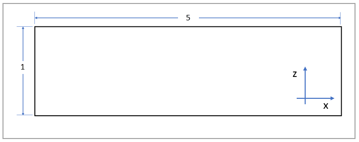
The domain consists of a cylinder (the pipe) with an inflow section of uniform prescribed velocity, an outflow section of prescribed pressure and the lateral surface boundary (pipe wall) with a non-slip condition. The domain size and relevant quantities are shown in Figure 145. For this test case, all units of measure are consistent (length = m, time = s, mass = kg, force = N, pressure = Pa).
| Material Properties | Geometric Properties | Loading |
|---|---|---|
|
Fluid: Fluid density ρ = 1 kg/m3 Inflow axial velocity at pipe inlet U = 1 m/s Flow dynamic viscosity μ = 0.2 N s/m2 | Mesh size: Boundary elements size: 0.04 Anisotropic elements added to Boundary Layer: 3 Geometry: Pipe Radius R = 0.5 m Pipe Length L = 5 m |
Fluid: Outflow pressure Pout = 0 N/m2 |
Analysis Assumptions and Modeling Notes
The Hagen-Poiseuille flow model provides a closed form relationship between flow speed and pression gradient for an incompressible (Newtonian) fluid in laminar flow. The Poiseuille flow is one of the few cases in which (for the given hypotheses) the Navier-Stokes equations provide an analytical solution. For the case of a pipe (3D problem) with constant section, assuming a completely developed laminar boundary layer, the axial velocity distribution in cylindrical coordinates is
 | (17) |
where  is the distance from the pipe axis in radial coordinates,
  is the pipe diameter,
  is the flow dynamic viscosity, and
  is the constant pressure gradient along the pipe axis. The maximum value of
the velocity profile is, then
is the constant pressure gradient along the pipe axis. The maximum value of
the velocity profile is, then
 | (18) |
In this study, a uniform velocity profile with  is imposed at the pipe inlet. After the boundary layer fully develops, the
velocity distribution will remain constant in every section along the pipe length. The
pressure jump at each section of the pipe is, then
is imposed at the pipe inlet. After the boundary layer fully develops, the
velocity distribution will remain constant in every section along the pipe length. The
pressure jump at each section of the pipe is, then
 | (19) |
where  is the distance from the pipe outlet and the pressure at the pipe outlet
 is imposed. The distribution of
  will be compared between the outlet section and section at
  . After verifying that the boundary layer has been fully developed and that
 is the same at both sections, the value of
  will be compared to the analytical result.
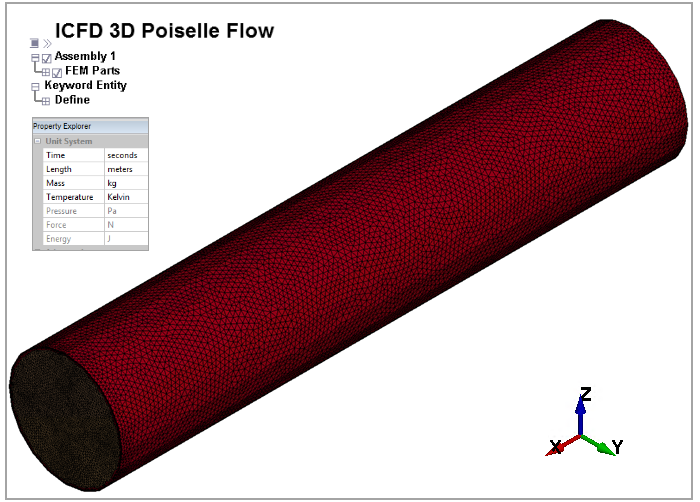
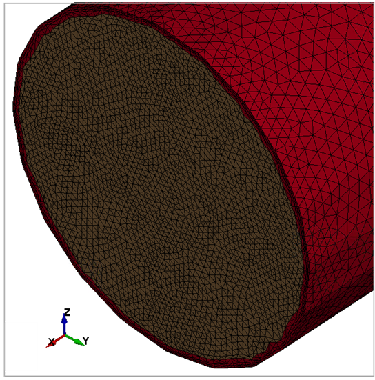
A picture of the domain mesh is shown in Figure 146, while Figure 147 shows a detail of the mesh close to the pipe inlet. The elements in red belong to the pipe boundary layer. LS-DYNA uses tetrahedral elements in 3D to mesh the fluid domain. The discretization has been obtained using LS-DYNA's automatic mesh generator.
Results Comparison
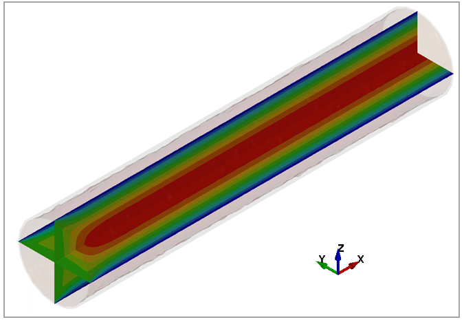
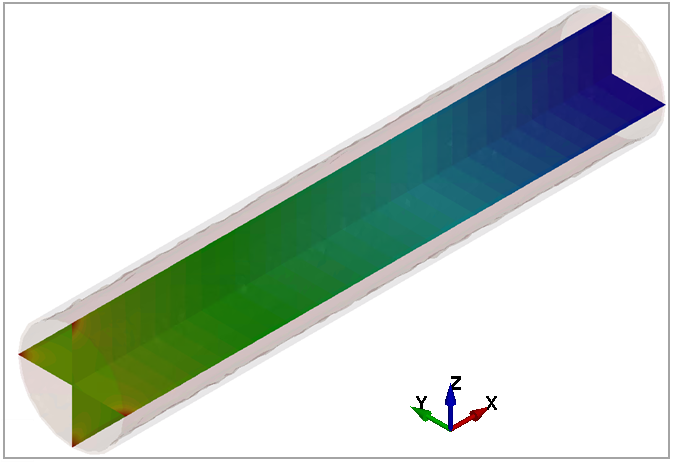
Figure 148 shows the flow velocity fringes in the axial direction of the pipe through two sections orthogonal to the y- and z-directions. After the boundary layer fully develops, the velocity profile is parabolic for each section, equal to 0 on the pipe wall and maximum on the axis, in accordance with the flow model. The flow is axially symmetric and constant along the pipe axis.
Figure 149 shows the flow pressure
fringes in the axial direction of the pipe through two sections orthogonal to the y- and
z-directions. It is possible to appreciate how the pression changes linearly along the pipe
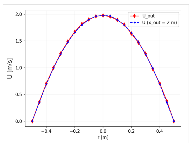
axis, after the full development of the boundary layer. Finally Figure 150 shows a comparison of the
velocity profiles between the outlet section and section at  . This is further confirmation that at the boundary layer is completely developed.
The results table below shows a comparison of  between the present analysis and the reference (analytical value).
| Results | Target | LS-DYNA | Error (%) |
|---|---|---|---|
|
| 12.65 | 12.92 | 2.11% |