Using this feature, you can apply translational (force) or rotational (moment) loads on entities in all three directions.
Forces can be applied by two different features. The Uniform feature applies the stated force at all selected entities. For example with curves, the Uniform feature will apply the full force to all nodes attached to the curve. The Total feature means that the force gets distributed among all the nodes of the selected entities according to FEA concepts as described below.
Distributed Forces Theory
Total forces are distributed as described below, depending on the entity type.
By Curve
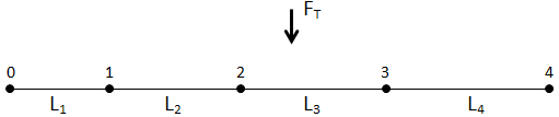
The total Force 'FT ' can be applied on a curve as shown below. Applying the load to a geometry entity simplifies the process for you and keeps the load information at the geometry level so the mesh can be regenerated without losing the setup information.
Nodes are numbered 0, 1, 2, and so on. Elements between the nodes have lengths L1, L2 and so on. The total length is LT.
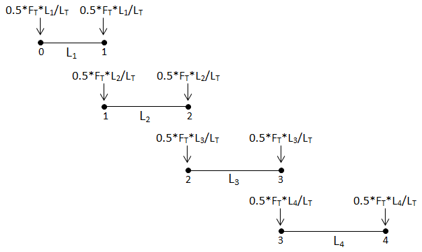
Then the force on the Nodes, as per FEA concepts, is distributed linearly in proportion to the Element length as shown in the figure below.
For a Linear distribution, the load at each node is calculated as follows.
Node 0: F0 = 0.5 * FT * (L1 / LT)
Node 1: F1 = 0.5 * FT * (L1 / LT) + 0.5 * FT * (L2 / LT)
Node 2: F2 = 0.5 * FT * (L2 / LT) + 0.5 * FT * (L3 / LT)
Node 3: F3 = 0.5 * FT * (L3 / LT) + 0.5 * FT * (L4 / LT)
Node 4: F4 = 0.5 * FT * (L4 / LT)
In general, the force at any Node is: Fi = Sum [FT * (Lj / LT) * (1 / Nj)], where i is the node number, j is the element number, Lj is the length of element j, and Nj is the number of Nodes attached to element j.
As a check, if you add the individual node forces, F0 + F1 + F2 + F3 + F4 , then the result equals FT .
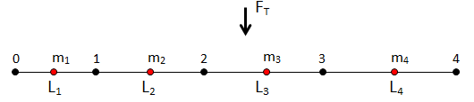
By Mesh Elements
You can also apply loads directly to the elements (select the elements directly rather than the geometry entities). This can occur, for example, if you do not have the geometry in a particular model or area of a model. In this case, the load is distributed element-by-element using a Quadratic distribution as shown.
Node numbers and element lengths are defined as before. In addition, each element has a mid-side node labeled m1, m2, and so on.
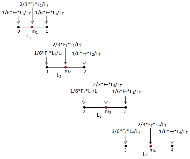
The Quadratic Load distribution, as per FEA concepts on an element-by-element basis is shown in Figure 33: Quadratic Load Distribution.
The distribution of the Total Force, FT, at the boundary nodes is as follows:
Node 0: F0q = 1/6 * FT * (L1 / LT)
Node 1: F1q = 1/6 * FT * (L1 / LT) + 1/6 * FT * (L2 / LT)
Node 2: F2q = 1/6 * FT * (L2 / LT) + 1/6 * FT * (L3 / LT)
Node 3: F3q = 1/6 * FT * (L3 / LT) + 1/6 * FT * (L4 / LT)
Node 4: F4q = 1/6 * FT * (L4 / LT)
And the distribution at mid-side nodes is:
Node m1: Fm1 = 2/3 * FT * (L1 / LT)
Node m2: Fm2 = 2/3 * FT * (L2 / LT)
Node m3: Fm3 = 2/3 * FT * (L3 / LT)
Node m4: Fm4 = 2/3 * FT * (L4 / LT)
As in the previous case of linear distribution, you can check the total Force by adding the individual nodal forces:
FT = F0q + F1q + F2q + F3q + F4q + Fm1 + Fm2 + Fm3 + Fm4.
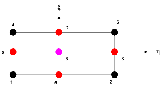
By Surface
If you choose to set a load on a surface entity, then the load distribution follows the Nine Node, Two Dimension, Lagrange distribution. See the Figure 34: QUAD 9 Element for an illustration.
Nine nodes are identified: N1-N4 at the corners; N5-N8 at the mid-sides; and N9 in the middle. The symbols ξ and η define a local coordinate system for the development of the load distribution, and vary from –1 to +1 over the surface of the element.
The Shape function for the distribution at a Corner Node is:

At a Mid-Side Node, the Shape function for the distribution is:

And finally, the Shape function for the Middle Node load distribution is:

Suppose a Force F is uniformly distributed over the whole Area. Then the pressure is P = F / 4. (Because in the ξ-η coordinate system the area of the surface is 4.)
To find the Consistent Load at each Node, we must integrate the Shape function over the surface area:
Consistent Load at Node 1 = L1:

Consistent Load at Node 5 = L5:

Consistent Load at Node 9 = L9:

Now F = 4P.
Substituting this value in the above equations we get the Consistent Load as
L1 = F / 36
L5 = F / 9
L9 = 4F / 9
By symmetry, the Consistent Load on all corner nodes N1, N2, N3, and N4 are equal.
Similarly, the Consistent Load on all mid-side nodes N5, N6, N7, and N8 are equal.
As with the Linear and Quadratic distributions, a check against the Total can be performed.
The sum of the Consistent Loads = 4 * L1 + 4 * L5 + L9
= F / 9 + 4F / 9 + 4F / 9
= FT
Note: A similar process for calculating the Consistent Load on a QUAD8 element load distribution is available. Again, the output file is generated thru the "Solve Options" Tab, and during output, the distributed load information will be written out according to the selected solver's published format.