


The discrete ordinates (DO) radiation model solves the radiative
transfer equation (RTE) for a finite number of discrete solid angles,
each associated with a vector direction  fixed in the global Cartesian system (x, y, z). The
DO model solves for as many transport equations as there are directions
fixed in the global Cartesian system (x, y, z). The
DO model solves for as many transport equations as there are directions  . The solution method is identical to that
used for the fluid flow and energy equations.
. The solution method is identical to that
used for the fluid flow and energy equations.
The DO Model Equations
The DO model considers the radiative transfer equation (RTE)
in the direction  as a field equation. Thus, Equation 40–107 is
written as
as a field equation. Thus, Equation 40–107 is
written as
 | (40–107) |
Angular Discretization and Pixelation
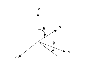
Each octant of the angular space 4 at any spatial location is discretized into N x N solid angles of extent, called control angles. The angles are the polar and azimuthal angles respectively, and are measured with respect to the global Cartesian system (x, y, z) as shown in Figure 40.2: The Angular Coordinate System. The theta and phi extents of the control angle, are constant. In two-dimensional calculations, only four octants are solved due to symmetry, making a total of directions in all. In three-dimensional calculations, a total of directions are solved. In the case of the non-gray model equations are solved for each band.
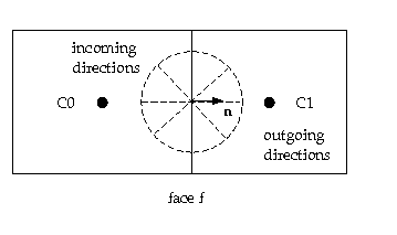
When Cartesian meshes are used, it is possible to align the global angular discretization with the control volume face, as shown in Figure 40.3: The Face with No Control Angle Overhang. For generalized unstructured meshes however, control volume faces do not in general align with the global angular discretization, as shown in Figure 40.4: The Face with Control Angle Overhang leading to the problem of control angle overhang.
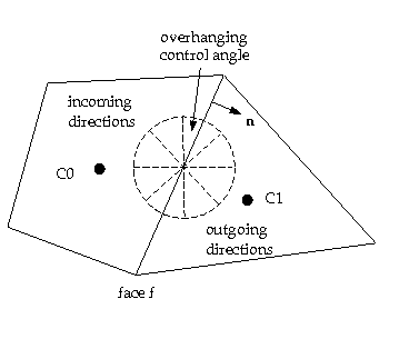
Essentially, control angles can straddle the control volume faces, so that they are partially outgoing to the face. Figure 40.4: The Face with Control Angle Overhang shows a 3D example of a face with control angle overhang.
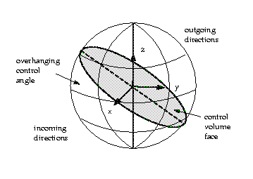
The control volume face cuts the sphere representing the angular space at an arbitrary angle. The line of intersection is a great circle. Control angle overhang may also occur as a result of reflection and refraction. It is important in these cases to correctly account for the overhanging fraction. This is done through the use of pixelation.
Each overhanging control angle is divided into  pixels, as shown
in Figure 40.6: The Pixelation of Control Angle
pixels, as shown
in Figure 40.6: The Pixelation of Control Angle
The energy contained in each pixel is then treated as incoming or outgoing to the face. The influence of overhang can thus be accounted for within the pixel resolution. Ansys Icepak allows you to choose the pixel resolution. For problems involving gray-diffuse radiation, the default pixelation of 1 X 1 is usually sufficient. For problems involving symmetry, periodic, specular, or semi-transparent boundaries, a pixelation of 3 X 3 is recommended. You should be aware, however that increasing the pixelation adds to the cost of computation.