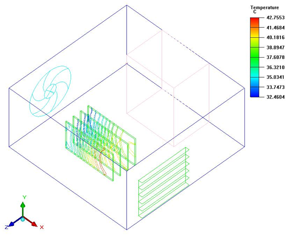
Contours are representations of the variation of a specified variable drawn as lines or solid bands. An individual contour follows a single value of a variable and can curve around or through objects. Contour plots are used to examine how a variable changes locally or throughout the model, and are often useful for locating severe gradients and conditions (for example, hot spots on the surfaces of objects).

Line contours (for example, Figure 37.17: Contour Plot) resemble topological maps. Solid contours can be specified as either smooth or bands. For smooth contours the colors change in continuous gradations from one boundary of the contour to the other. For banded contours, the colors change abruptly at the contour boundaries.

Figure 37.17: Contour Plot

Overview of Defining a Contour Plot

If you have selected Show contours as the type of display to be shown on an object face, plane cut, or isosurface (in the Object face, Plane cut, or Isosurface panel), you can click the associated Parameters button to modify the definition of the contour plot. Figure 37.18: The Object face contours Panel shows an example of the Object face contours panel.

Figure 37.18: The Object face contours Panel

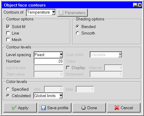
In the Object face contours panel, the Plane cut contours panel, or the Isosurface contours panel, you can specify the variable to be plotted, the type of contour plot (line or solid), the color levels for the plot, and several characteristics of the contour lines or solid contours. When you are satisfied with the new settings, click Apply to see the results in the graphics window.

Selecting the Variable to be Plotted

To choose the variable to be displayed, select the desired variable (for example, Temperature) from the Variable drop-down list. The available variables are described in Variables for Postprocessing and Reporting.

Specifying a Line or Solid Contour Plot

To specify whether you want a line contour plot or a solid contour plot (or both), turn on the Solid or Line option for Contour options. If you select both, the contours will be displayed as solid color bands with lines superimposed on them.

For line contour plots, you will specify how the line color is determined, and for solid contour plots you will specify the shading. For both, you will also specify how the spacing or band width between contours is determined.

Constant or Variable Color for a Line Contour Plot

There are two ways to color the lines on a line contour plot. To vary the color of the lines based on the value of the variable being plotted, select the Variable option in the Line color drop-down list. To have a single color for all the lines, select the Fixed option in the Line color drop-down list and then specify a color in the Color drop-down color palette.

Shading for a Solid Contour Plot

There are two ways to shade the contours on a solid contour plot. To vary the colors smoothly in continuous gradations from one boundary of the contour to the other, select the Smooth option under Shading options. For plane cut contours, you can view smooth shading in 3D, click on 3D and enter scale and ref values. The scale values are arbitrary numbers that aid in visualization. The ref value, enabled for 3D plotting only, refers to the user set ambient condition value of a physical quantity under consideration. Changing the ref value repositions the plane surface position such that the base of 3D contour would have its value set as the ref value. To have the colors change abruptly at the contour boundaries, select the Banded option.

Specifying the Line Spacing or Band Width

For both line and solid contour plots, there are three ways to specify the line spacing or band width:

Displaying the Value of a Variable on a Line

To display the value of a variable on a line, click Display and enter a number in the Interval text box. Interval represents the number of sections of a line where the values will be displayed. The default value is 4. The format or precision of these values can be controlled using the Display section of the Preferences panel.

Specifying the Color Levels

The color spectrum for a line or solid contour plot is distributed across a range of values for the variable being plotted. There are two ways to specify the minimum and maximum limits for this range:

Saving a Contour Plot

After creating a contour plot, you can save the contour data to a file so that you can read it back into Ansys Icepak as a profile. This is useful if you have solved a large complicated problem and you want to zoom in to a specific region of your model and solve this region in more detail. You can use the contour data as the boundary conditions for the region you want to study in more detail, and then calculate a solution only for this region.

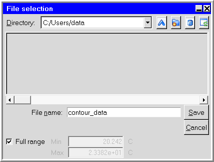
To save contour data, create a contour plot for one of the boundaries of the region to be studied in detail, and then click Save profile in the associated contour panel (for example, Figure 37.18: The Object face contours Panel). Enter a name for the contour plot in the resulting File selection dialog box. For Object face (facet) objects, you can save the full range of data or enter Min and Max values to save the specified range. Click Accept to save the data. You can then create a wall or an opening at the same boundary of the region to be studied in detail. To use the contour data as the boundary condition for the wall or opening, define a spatial profile on the wall or opening using the contour data. (For information on specifying a spatial profile for an opening, see Openings; for a wall, see Walls.)

Figure 37.19: Arrow Styles: 2D arrow heads and Rhomboid