


Ansys Fluent implements a finite-volume method for computing the resonance frequencies and natural acoustic modes for any enclosure. Sound wave propagation, reflection, diffraction, and convection are taken into account. The formulation requires an input of the mean flow obtained from a steady-state solution, together with prescribed boundary conditions. The method involves solving the Linearized Navier-Stokes Equations with the iterative Implicitly Restarted Arnoldi method to find the eigenvalues (frequencies) and eigenvectors (mode shapes of the pressure and velocity fluctuations).
The following limitations apply to the modal analysis model currently implemented in Ansys Fluent:
The modal analysis model is applicable to a steady-state, compressible ideal-gas solution.
The modal analysis model is available for the double precision, serial Ansys Fluent version.
The modal analysis model treats all domain boundaries as sound reflecting boundaries. Fluid particles can enter and leave the domain but acoustic waves are reflected.
The system of 3D Linearized Navier-Stokes equations, in a Cartesian coordinate system are:
 | (13–1) |
 | (13–2) |
 | (13–3) |
where  is the molecular
stress tensor
is the molecular
stress tensor
 | (13–4) |
and the subscript  represents the mean values, and superscript
  represents the acoustic
fluctuation about this mean (for example,
represents the acoustic
fluctuation about this mean (for example,  ). Note that
a thermally perfect ideal gas is assumed.
). Note that
a thermally perfect ideal gas is assumed.  is the Kronecker delta function,
  is the molecular viscosity,
  is the conductive
heat diffusivity coefficient,
is the conductive
heat diffusivity coefficient,  and
and  are the specific
heats at constant volume and constant pressure, respectively.
are the specific
heats at constant volume and constant pressure, respectively.
The mean flow conditions are first solved from a steady-state
solution of the Reynolds-Averaged Navier-Stokes equations. The fluctuating
quantities are assumed harmonic functions in time, so that  , where
  . Substituting this into the linearized Navier-Stokes
gives
. Substituting this into the linearized Navier-Stokes
gives
 | (13–5) |
The Jacobians  and
and  are the direct linearizations of the discretized
flow equations.
are the direct linearizations of the discretized
flow equations.
With  , this
system of equations can be written as:
, this
system of equations can be written as:
 | (13–6) |
where  and
and  ,
,  is the solution of the eigenvalues
problem.
is the solution of the eigenvalues
problem.  is the eigenvector
for the complex eigenvalue
is the eigenvector
for the complex eigenvalue  . The
proper acoustic response of boundaries is included in the modal analysis
model [1].
. The
proper acoustic response of boundaries is included in the modal analysis
model [1].
Equation 13–6 is an eigen-system and the iterative Implicitly Restarted Arnoldi method is use to compute a small set of eigenvalues and eigenvectors in a limited range of interest. The Implicitly Restarted Arnoldi method uses the ARPACK package (http://www.caam.rice.edu/software/ARPACK/), which is a collection of Fortran 77 subroutines designed to solve large-scale eigenvalue problems.
Make sure you first enable beta feature access, as described in Introduction. The procedure for computing the resonance frequencies and acoustic modes using the modal analysis model in Ansys Fluent is as follows:
Calculate a converged steady-state compressible RANS solution.
Enable the Modal Analysis acoustics model.
 Setup → Models →
Acoustics
Setup → Models →
Acoustics Edit...
Set the associated Model Constants in the Acoustics Model dialog box.
Compute the resonance frequencies and acoustic modes by clicking the Solve button.
Postprocess the acoustic modes.
 Postprocessing → Graphics → Contours → Edit...
Under Model Constants in the Acoustics Model dialog box (Figure 13.1: The Acoustics Model Dialog Box), specify the relevant acoustic parameters used by the model.
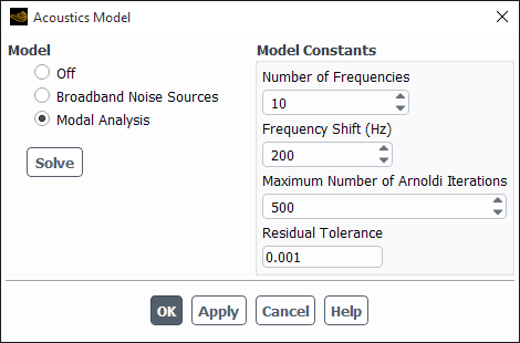
- Number of Frequencies
is the requested maximum number of eigenvalues (natural acoustic frequencies). The default of 30.
- Frequency Shift
is the frequency around which the eigenvalues will be solved. When the frequency shift is zero, the Arnoldi algorithm computes the eigenvalues around the smallest magnitude (SM). The default is 200Hz.
- Maximum Number of Arnoldi Iterations
: the Implicitly Restarted Arnoldi Method is terminated after this many iterations if not converged. The default is 500.
- Residual Tolerance
is the convergence criterion for the Arnoldi algorithm. The default is 0.001.
Postprocessing of the acoustic modes is accomplished by selecting the Acoustics category in the postprocessing dialog boxes:
Acoustic Pressure Mode n
where n ranges from 1 to 10.