UDFs are called at predetermined times in the Ansys Fluent solution process. However, they can
also be executed asynchronously (or "on demand") using a
DEFINE_ON_DEMAND UDF. If a
DEFINE_EXECUTE_AT_END UDF is used, then Ansys Fluent calls the function at
the end of an iteration. A DEFINE_EXECUTE_AT_EXIT is called at the end
of an Ansys Fluent session while a DEFINE_EXECUTE_ON_LOADING is called
whenever a UDF compiled library is loaded. Understanding the context in which UDFs are called
within Ansys Fluent's solution process may be important when you begin the process of writing UDF
code, depending on the type of UDF you are writing. The solver contains call-outs that are linked
to user-defined functions that you write. Knowing the sequencing of function calls within an
iteration in the Ansys Fluent solution process can help you determine which data are current and
available at any given time.
For more information, see the following:
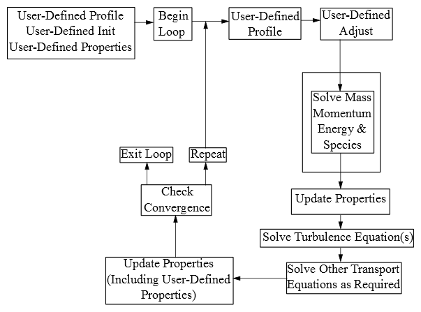
The solution process for the pressure-based segregated solver (Figure 1.2: Solution Procedure for the Pressure-Based Segregated Solver) begins with a two-step initialization sequence that is
executed outside of the solution iteration loop. This sequence begins by initializing equations
to user-entered (or default) values taken from the Ansys Fluent user interface. Next,
PROFILE UDFs are called, followed by a call to
INIT UDFs. Initialization UDFs overwrite initialization values that
were previously set.
The solution iteration loop begins with the execution of
ADJUST UDFs (note that this is true for the first iteration loop only;
for subsequent iteration loops, PROFILE UDFs are executed prior to
ADJUST UDFs). Next, momentum equations for u, v, and w velocities are
solved sequentially, followed by mass continuity and velocity updates. Subsequently, the energy
and species equations are solved, followed by turbulence and other scalar transport equations,
as required. Note that PROFILE and SOURCE UDFs
are called by each "Solve" routine for the variable currently under consideration
(for example, species, velocity).
After the conservation equations, properties are updated, including
PROPERTY UDFs. Thus, if your model involves the gas law, for example,
the density will be updated at this time using the updated temperature (and pressure and/or
species mass fractions). A check for either convergence or additional requested iterations is
done, and the loop either continues or stops.
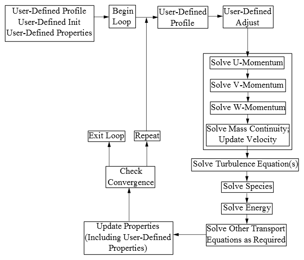
The solution process for the pressure-based coupled solver (Figure 1.3: Solution Procedure for the Pressure-Based Coupled Solver) begins with a two-step initialization
sequence that is executed outside of the solution iteration loop.
This sequence begins by initializing equations to user-entered (or
default) values taken from the Ansys Fluent user interface. Next, PROFILE UDFs are called, followed by a call to INIT UDFs. Initialization UDFs overwrite initialization
values that were previously set.
The solution iteration loop begins with the execution of
ADJUST UDFs (note that this is true for the first iteration loop
only; for subsequent iteration loops, PROFILE UDFs are executed prior
to ADJUST UDFs). Next, Ansys Fluent solves the governing equations of
continuity and momentum in a coupled fashion, which is simultaneously as a set, or vector, of
equations. Energy, species transport, turbulence, and other transport equations as required are
subsequently solved sequentially, and the remaining process is the same as the pressure-based
segregated solver.
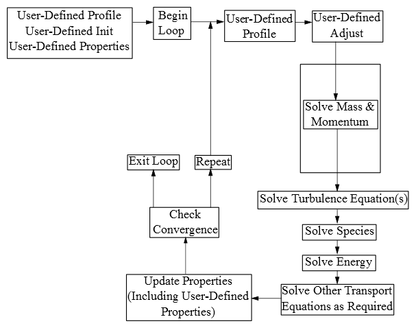
As is the case for the other solvers, the solution process for
the density-based solver (Figure 1.4: Solution Procedure for the Density-Based Solver) begins with a two-step initialization sequence that is executed
outside the solution iteration loop. This sequence begins by initializing
equations to user-entered (or default) values taken from the Ansys Fluent user
interface. Next, PROFILE UDFs are called,
followed by a call to INIT UDFs. Initialization
UDFs overwrite initialization values that were previously set.
The solution iteration loop begins with the execution of
ADJUST UDFs (note that this is true for the first iteration loop
only; for subsequent iteration loops, PROFILE UDFs are executed prior
to ADJUST UDFs). Next, Ansys Fluent solves the governing equations of
continuity and momentum, energy, and species transport in a coupled fashion, which is
simultaneously as a set, or vector, of equations. Turbulence and other transport equations as
required are subsequently solved sequentially, and the remaining process is the same as the
pressure-based segregated solver.