Chapter 1: Introduction to Using Ansys Fluent in Ansys Workbench: Fluid Flow and Heat Transfer in a Mixing Elbow

This tutorial is divided into the following sections:

1.1. Introduction

This tutorial illustrates using Ansys Fluent fluid flow systems in Ansys Workbench to set up and solve a three-dimensional turbulent fluid-flow and heat-transfer problem in a mixing elbow. It is designed to introduce you to the Ansys Workbench tool set using a simple geometry. Guided by the steps that follow, you will create the elbow geometry and the corresponding computational mesh using the geometry and meshing tools within Ansys Workbench. You will use Ansys Fluent to set up and solve the CFD problem, then visualize the results in both Ansys Fluent and in the CFD-Post postprocessing tool. Some capabilities of Ansys Workbench (for example, duplicating fluid flow systems, connecting systems, and comparing multiple data sets) are also examined in this tutorial.

This tutorial demonstrates how to do the following:

Launch Ansys Workbench.
Create a Fluent fluid flow analysis system in Ansys Workbench.
Create the elbow geometry using Ansys DesignModeler.
Create the computational mesh for the geometry using Ansys Meshing.
Set up the CFD simulation in Ansys Fluent, which includes:
- Setting material properties and boundary conditions for a turbulent forced-convection problem.
- Initiating the calculation with residual plotting.
- Calculating a solution using the pressure-based solver.
- Examining the flow and temperature fields using Ansys Fluent and CFD-Post.
Create a copy of the original Fluent fluid flow analysis system in Ansys Workbench.
Change the geometry in Ansys DesignModeler, using the duplicated system.
Regenerate the computational mesh.
Recalculate a solution in Ansys Fluent.
Compare the results of the two calculations in CFD-Post.

1.2. Prerequisites

This tutorial assumes that you have little to no experience with Ansys Workbench, Ansys DesignModeler, Ansys Meshing, Ansys Fluent, or CFD-Post, and so each step will be explicitly described.

1.3. Problem Description

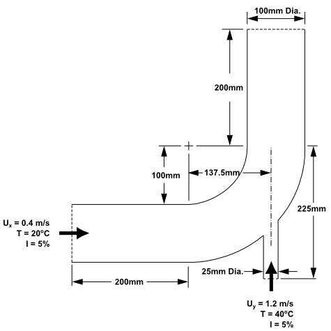
The problem to be considered is shown schematically in Figure 1.1: Problem Specification. A cold fluid at 293.15 K flows into the pipe through a large inlet and mixes with a warmer fluid at 313.15 K that enters through a smaller inlet located at the elbow. The mixing elbow configuration is encountered in piping systems in power plants and process industries. It is often important to predict the flow field and temperature field in the area of the mixing region in order to properly design the junction.

Note: Because the geometry of the mixing elbow is symmetric, only half of the elbow must be modeled.

Figure 1.1: Problem Specification

Note: The functionality to create named selections exists in both Ansys DesignModeler and Ansys Meshing. For the purposes of this tutorial, named selections are created in Ansys Meshing since the meshing application provides more comprehensive and extensive named selection functionality.

1.4. Setup and Solution

To help you quickly identify graphical user interface items at a glance and guide you through the steps of setting up and running your simulation, the Ansys Fluent Tutorial Guide uses several type styles and mini flow charts. See Typographical Conventions Used In This Manual for detailed information.

The following sections describe the setup and solution steps for this tutorial:

1.4.1. Preparation

Download the workbench_elbow.zip file here .
Unzip workbench_elbow.zip to your working folder. This file contains a folder, workbench_elbow, that holds the following items:
- two geometry files, elbow-geometry.agdb and elbow-geometry.stp

Note: Ansys Fluent tutorials are prepared using Ansys Fluent on a Windows system. The screen shots and graphic images in the tutorials may be slightly different than the appearance on your system, depending on the operating system or graphics card.

1.4.2. Creating a Fluent Fluid Flow Analysis System in Ansys Workbench

In this step, you will start Ansys Workbench, create a new Fluent fluid flow analysis system, then review the list of files generated by Ansys Workbench.

From the Windows Start menu, select Start > Ansys 2024 R2 > Workbench 2024 R2 to start a new Ansys Workbench session.
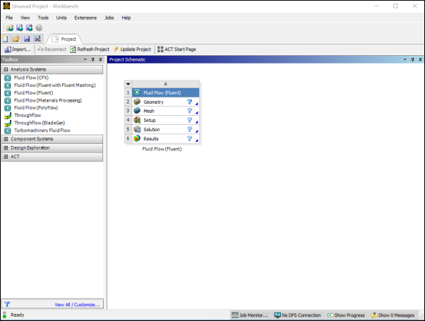
This displays the Ansys Workbench application window, which has the Toolbox on the left and the Project Schematic to its right. Various supported applications are listed in the Toolbox and the components of the analysis system will be displayed in the Project Schematic.
Note: Depending on which other products you have installed, the analysis systems that appear may differ from those in the figures that follow in this tutorial.
Create a new Fluent fluid flow analysis system by double-clicking the Fluid Flow (Fluent) option under Analysis Systems in the Toolbox.
Tip: You can also drag-and-drop the analysis system into the Project Schematic. A green dotted outline indicating a potential location for the new system initially appears in the Project Schematic. When you drag the system to one of the outlines, it turns into a red box to indicate the chosen location of the new system.
Figure 1.2: Ansys Workbench with a New Fluent-Based Fluid Flow Analysis System
Name the analysis.
1. Double-click the Fluid Flow (Fluent) label underneath the analysis system (if it is not already highlighted).
2. Enter elbow for the name of the analysis system.
Save the project.
1. In Ansys Workbench, under the File menu, select Save.
  File → Save
  This displays the Save As dialog box, where you can browse to your working folder and enter a specific name for the Ansys Workbench project.
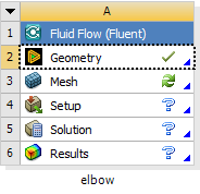
2. In your working directory, enter elbow-workbench as the project File name and click the Save button to save the project. Ansys Workbench saves the project with a .wbpj extension and also saves supporting files for the project.
  Note that the fluid flow analysis system is composed of various cells (Geometry, Mesh, etc.) that represent the workflow for performing the analysis. Ansys Workbench is composed of multiple data-integrated and native applications in a single, seamless project flow, where individual cells can obtain data from other cells and provide data to other cells. As a result of this constant flow of data, a cell’s state can quickly change. Ansys Workbench provides a visual indication of a cell’s state at any given time via icons on the right side of each cell. Brief descriptions of the various states are provided below:
  - Unfulfilled ( ) indicates that required upstream data does not exist. For example, when you first create a new Fluid Flow (Fluent) analysis system, all cells downstream of the Geometry cell appear as Unfulfilled because you have not yet specified a geometry for the system.
  - Refresh Required ( ) indicates that upstream data has changed since the last refresh or update. For example, after you assign a geometry to the geometry cell in your new Fluid Flow (Fluent) analysis system, the Mesh cell appears as Refresh Required since the geometry data has not yet been passed from the Geometry cell to the Mesh cell.
  - Attention Required ( ) indicates that the current upstream data has been passed to the cell, however, you must take some action to proceed. For example, after you launch Ansys Fluent from the Setup cell in a Fluid Flow (Fluent) analysis system that has a valid mesh, the Setup cell appears as Attention Required because additional data must be entered in Ansys Fluent before you can calculate a solution.
  - Update Required ( ) indicates that local data has changed and the output of the cell must be regenerated. For example, after you launch Ansys Meshing from the Mesh cell in a Fluid Flow (Fluent) analysis system that has a valid geometry, the Mesh cell appears as Update Required because the Mesh cell has all the data it must generate an Ansys Fluent mesh file, but the Ansys Fluent mesh file has not yet been generated.
  - Up To Date ( ) indicates that an update has been performed on the cell and no failures have occurred or that an interactive calculation has been completed successfully. For example, after Ansys Fluent finishes performing the number of iterations that you request, the Solution cell appears as Up-to-Date.
  - Interrupted, Update Required ( ) indicates that you have interrupted an update (or canceled an interactive calculation that is in progress). For example, if you select the Cancel button in Ansys Fluent while it is iterating, Ansys Fluent completes the current iteration and then the Solution cell appears as Interrupted, Update Required.
  - Input Changes Pending ( ) indicates that the cell is locally up-to-date, but may change when next updated as a result of changes made to upstream cells. For example, if you change the Mesh in an Up-to-Date Fluid Flow (Fluent) analysis system, the Setup cell appears as Refresh Required, and the Solution and Results cells appear as Input Changes Pending.
  - Pending ( ) indicates that a batch or asynchronous solution is in progress. When a cell enters the Pending state, you can interact with the project to exit Workbench or work with other parts of the project. If you make changes to the project that are upstream of the updating cell, then the cell will not be in an up-to-date state when the solution completes.
  For more information about cell states, see the Workbench User's Guide.
View the list of files generated by Ansys Workbench.
Ansys Workbench allows you to easily view the files associated with your project using the Files view. To open the Files view, select the Files option under the View menu at the top of the Ansys Workbench window.
View → Files
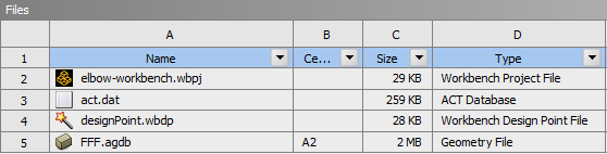
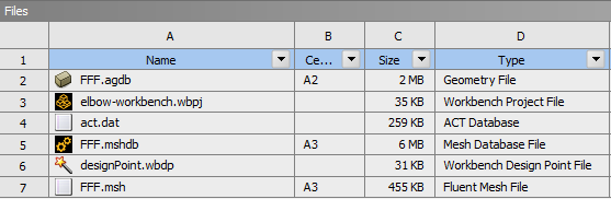
Figure 1.3: Ansys Workbench Files View for the Project After Adding a Fluent-Based Fluid Flow Analysis System

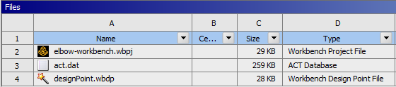
In the Files view, you will be able to see the name and type of file, the ID of the cell that the file is associated with, the size of the file, the location of the file, and other information. For more information about the Files view, see the Workbench User's Guide.
Note: The sizes of the files listed may differ slightly from those portrayed in Figure 1.3: Ansys Workbench Files View for the Project After Adding a Fluent-Based Fluid Flow Analysis System.
From here, you will create the geometry described in Figure 1.1: Problem Specification, and later create a mesh and set up a fluid flow analysis for the geometry.

1.4.3. Creating the Geometry in Ansys DesignModeler

For the geometry of your fluid flow analysis, you can create a geometry in Ansys DesignModeler, Ansys SpaceClaim Direct Modeler, or import the appropriate geometry file. In this step, you will create the geometry in Ansys DesignModeler, then review the list of files generated by Ansys Workbench.

Important: Note the Attention Required icon ( ) within the Geometry cell for the system. This indicates that the cell requires data (for example, a geometry). Once the geometry is defined, the state of the cell will change accordingly. Likewise, the state of some of the remaining cells in the system will change.

Note: If you would rather not create the geometry in Ansys DesignModeler, you can import a pre-existing geometry by right-clicking the Geometry cell and selecting the Import Geometry option from the context menu. From there, you can browse your file system to locate the elbow_geometry.agdb geometry file that is provided for this tutorial. If you do not have access to Ansys DesignModeler, you can use the elbow_geometry.stp file instead.

To learn how to create a mesh from the geometry you imported, go to Meshing the Geometry in the Ansys Meshing Application.

Start Ansys DesignModeler.
In the Ansys Workbench Project Schematic, right-click the Geometry cell in the elbow fluid flow analysis system to display the context menu, then select New DesignModeler Geometry.... This displays the Ansys DesignModeler application.
Set the units in Ansys DesignModeler.
When Ansys DesignModeler first appears, you should select desired system of length units to work from. For the purposes of this tutorial (where you will create the geometry in millimeters and perform the CFD analysis using SI units) set the units to Millimeter.
Units → Millimeter

Create the geometry.

The geometry for this tutorial (Figure 1.1: Problem Specification) consists of a large curved pipe accompanied by a smaller side pipe. Ansys DesignModeler provides various geometry primitives that can be combined to rapidly create geometries such as this one. You will perform the following tasks to create the geometry:

Create the bend in the main pipe by defining a segment of a torus.
Extrude the faces of the torus segment to form the straight inlet and outlet lengths.
Create the side pipe by adding a cylinder primitive.
Use the symmetry tool to reduce the model to half of the pipe assembly, thus reducing computational cost.

Create the main pipe:

Create a new torus for the pipe bend by choosing the Create → Primitives → Torus menu item from the menubar.
A preview of the torus geometry will appear in the graphics window. Note that this is a preview and the geometry has not been created yet. First you must specify the parameters of the torus primitive in the next step.
In the Details View for the new torus (Torus1), set Base Y Component to -1 by clicking the 1 to the right of FD10, Base Y Component, entering -1, and pressing Enter. This specifies the direction vector from the origin to the center of the circular cross-section at the start of the torus. In the same manner, specify Angle; Inner Radius; and Outer Radius as shown below.
Note: Enter only the value without the units of mm. They will be appended automatically because you specified the units previously.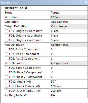
To create the torus segment, click the Generate button that is located in the Ansys DesignModeler toolbar.

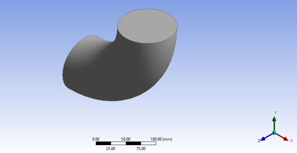
The Torus1 item appears in the Tree Outline view. If you want to delete this item, you can right-click it and select Delete from the context menu that opens.
Ensure that the selection filter is set to Faces. This is indicated by the Faces button appearing depressed in the toolbar and the appearance of the Face selection cursor, when you mouse over the geometry.
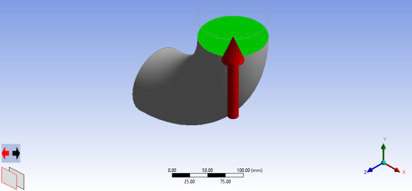
Select the top face (in the positive Y direction) of the elbow and click the Extrude button from the 3D Features toolbar.
In the Details View for the new extrusion (Extrude1), click Apply to the right of Geometry. This accepts the face you selected as the base geometry of the extrusion.
Click None (Normal) to the right of Direction Vector. Again, ensure that the selection filter is set to Faces, select the same face on the elbow to specify that the extrusion will be normal to the face and click Apply.
Enter 200 for FD1, Depth (>0) and click Generate.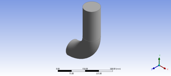

In a similar manner, create an extrusion of the other face of the torus segment to create the 200 mm inlet extension. You will probably find it helpful to rotate the view so that you can easily select the other face of the bend.

You can use the mouse buttons to change your view of the 3D image. The following table describes mouse actions that are available:

Table 1.1: DesignModeler View Manipulation Instructions

Action	Using Graphics Toolbar Buttons and the Mouse
Rotate view (vertical, horizontal)	After clicking the Rotate icon, , press and hold the left mouse button and drag the mouse. Dragging side to side rotates the view about the vertical axis, and dragging up and down rotates the view about the horizontal axis.
Translate or pan view	After clicking the Pan icon, , press and hold the left mouse button and drag the object with the mouse until the view is satisfactory.
Zoom in and out of view	After clicking the Zoom icon, , press and hold the left mouse button and drag the mouse up and down to zoom in and out of the view.
Box zoom	After clicking the Box Zoom icon, , press and hold the left mouse button and drag the mouse diagonally across the screen. This action will cause a rectangle to appear in the display. When you release the mouse button, a new view will be displayed that consists entirely of the contents of the rectangle.

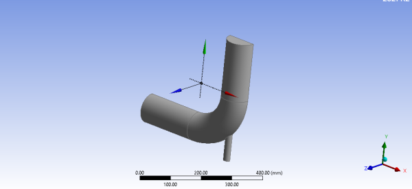
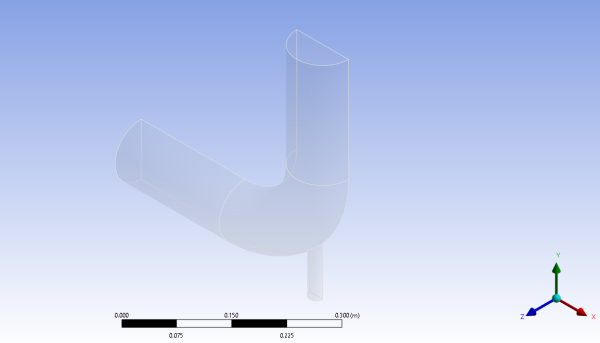
Clicking the Zoom to Fit icon, , will cause the object to fit exactly and be centered in the window.

After entering the extrusion parameters and clicking Generate, the geometry should appear as in Figure 1.4: Elbow Main Pipe Geometry.

Figure 1.4: Elbow Main Pipe Geometry

Next you will use a cylinder primitive to create the side pipe.

Choose Create → Primitives → Cylinder from the menubar.

In the Details View, set the parameters for the cylinder as follows and click Generate:

Setting	Value
BasePlane	`XYPlane`
FD3, Origin X Coordinate	`137.5`
FD4, Origin Y Coordinate	`-225`
FD5, Origin Z Coordinate	`0`
FD6, Axis X Component	`0`
FD7, Axis Y Component	`125`
FD8, Axis Z Component	`0`
FD10, Radius (>0)	`12.5`

The Origin Coordinates determine the starting point for the cylinder and the Axis Components determine the length and orientation of the cylinder body.

The final step in creating the geometry is to split the body on its symmetry plane which will halve the computational domain.
1. Choose Tools → Symmetry from the menu bar.
2. Select the XYPlane in the Tree Outline.
3. Click Apply next to Symmetry Plane 1 in the Details view.
4. Click Generate.
  
  The new surface created with this operation will be assigned a symmetry boundary condition in Fluent so that the model will accurately reflect the physics of the complete elbow geometry even though only half of it is meshed.
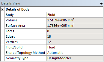
Specify the geometry as a fluid body.
1. In the Tree Outline, open the 1 Part, 1 Body branch and select Solid.
2. In the Details View of the body, change the name of the Body from Solid to Fluid.
3. In the Fluid/Solid section, select Fluid from the drop-down list.
4. Click Generate.

Tip: In addition to the primitives you used in this tutorial, Ansys DesignModeler offers a full suite of 2D sketching and 3D solid modeling tools for creating arbitrary geometry. Refer to the DesignModeler User's Guide for more information.

Close Ansys DesignModeler by selecting File → Close DesignModeler or by clicking the ‘X’ icon in the upper right-hand corner. Ansys Workbench automatically saves the geometry and updates the Project Schematic accordingly. The question mark in the Geometry cell is replaced by a check mark, indicating that there is a geometry now associated with the fluid flow analysis system.
View the list of files generated by Ansys Workbench by selecting View → Files.
Figure 1.5: Ansys Workbench Files View for the Project After Creating the Geometry

Note the addition of the geometry file (FFF.agdb, where FFF indicates a Fluent-based fluid flow system) to the list of files. If you had imported the geometry file provided for this tutorial rather than creating the geometry yourself, the elbow_geometry.agdb (or the elbow_geometry.stp) file would be listed instead.

1.4.4. Meshing the Geometry in the Ansys Meshing Application

Now that you have created the mixing elbow geometry, you must generate a computational mesh throughout the flow volume. For this section of the tutorial, you will use the Ansys Meshing application to create a mesh for your CFD analysis, then review the list of files generated by Ansys Workbench.

Important: Note the Refresh Required icon ( ) within the Mesh cell for the system. This indicates that the state of the cell requires a refresh and that upstream data has changed since the last refresh or update (such as an update to the geometry). Once the mesh is defined, the state of the Mesh cell will change accordingly, as will the state of the next cell in the system, in this case the Setup cell.

Open the Ansys Meshing application.
In the Ansys Workbench Project Schematic, double-click the Mesh cell in the elbow fluid flow analysis system (cell A3). This displays the Ansys Meshing application with the elbow geometry already loaded. You can also right-click the Mesh cell to display the context menu where you can select the Edit... option.
Figure 1.6: The Ansys Meshing Application with the Elbow Geometry Loaded
Create named selections for the geometry boundaries.
In order to simplify your work later on in Ansys Fluent, you should label each boundary in the geometry by creating named selections for the pipe inlets, the outlet, and the symmetry surface (the outer wall boundaries are automatically detected by Ansys Fluent).
1. Select the large inlet in the geometry that is displayed in the Ansys Meshing application.
  Tip:
  Use the Graphics Toolbar buttons and the mouse to manipulate the image until you can easily see the pipe openings and surfaces.
  To select the inlet, the Single select ( ) mode must be active.
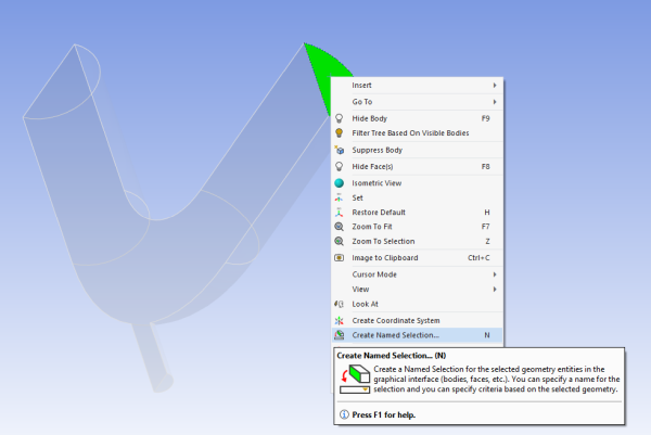
2. Right-click and select the Create Named Selection option.
  Figure 1.7: Selecting a Face to Name
  
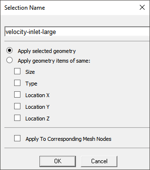
  This displays the Selection Name dialog box.
  Figure 1.8: Applying a Name to a Selected Face
3. In the Selection Name dialog box, enter velocity-inlet-large for the name and click OK.
4. Perform the same operations for:
  - The small inlet (velocity-inlet-small)
  - The large outlet (pressure-outlet)
  - The symmetry plane (symmetry).
  The named selections that you have created appear under the Named Selections item in the Outline view.
  Important: It is important to note that by using the strings “velocity inlet” and “pressure outlet” in the named selections (with or without hyphens or underscore characters), Ansys Fluent automatically detects and assigns the corresponding boundary types accordingly.
Create a named selection for the fluid body.
1. Change the selection filter to Body in the Graphics Toolbar ( ).
2. Click the elbow in the graphics display to select it.
3. Right-click, select the Create Named Selection option and name the body Fluid.
  By creating a named selection called Fluid for the fluid body you will ensure that Ansys Fluent automatically detects that the volume is a fluid zone and treats it accordingly.
Set basic meshing parameters for the Ansys Meshing application.
For this analysis, you will adjust several meshing parameters to obtain a finer mesh.
1. In the Outline view, select Mesh under Project/Model to display the Details of “Mesh” view below the Outline view.
  
  Important: Note that because the Ansys Meshing application automatically detects that you are going to perform a CFD fluid flow analysis using Ansys Fluent, the Physics Preference is already set to CFD and the Solver Preference is already set to Fluent.
2. Expand the Quality node to reveal additional quality parameters. Change Smoothing to High.
3. Add a Sizing control.
  1. With Mesh still selected in the Outline tree, click the elbow in the graphics display to select it.
  2. Right click in the graphics area and select Insert → Sizing from the context menu.
    
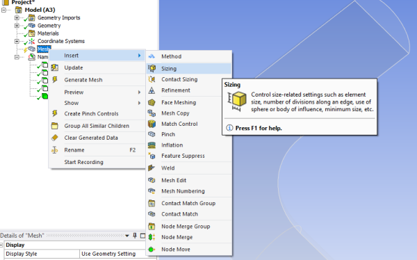
    A new Sizing entry appears under Mesh in the project Outline tree
  3. In the Outline tree, click the new Sizing control.
  4. Enter 6e-3 for Element Size and press Enter.
4. Click again Mesh in the Outline view and in the Details of “Mesh” view, expand the Inflation node to reveal additional inflation parameters. Change Use Automatic Inflation to Program Controlled.
Generate the mesh.
Right-click Mesh in the project Outline tree, and select Update in the context menu.
Figure 1.9: The Computational Mesh for the Elbow Geometry in the Ansys Meshing Application

Important: Using the Generate Mesh option creates the mesh, but does not actually create the relevant mesh files for the project and is optional if you already know that the mesh is acceptable. Using the Update option automatically generates the mesh, creates the relevant mesh files for your project, and updates the Ansys Workbench cell that references this mesh.

Note: Once the mesh is generated, you can view the mesh statistics by opening the Statistics node in the Details of “Mesh” view. This will display information such as the number of nodes and the number of elements.
Close the Ansys Meshing application.
You can close the Ansys Meshing application without saving it because Ansys Workbench automatically saves the mesh and updates the Project Schematic accordingly. The Refresh Required icon in the Mesh cell has been replaced by a check mark, indicating that there is a mesh now associated with the fluid flow analysis system.
View the list of files generated by Ansys Workbench.
View → Files
Figure 1.10: Ansys Workbench Files View for the Project After Mesh Creation

Note the addition of the mesh files (FFF.msh and FFF.mshdb) to the list of files. The FFF.msh file is created when you update the mesh, and the FFF.mshdb file is generated when you close the Ansys Meshing application.

1.4.5. Setting Up the CFD Simulation in Ansys Fluent

Now that you have created a computational mesh for the elbow geometry, you will set up a CFD analysis using Ansys Fluent, then review the list of files generated by Ansys Workbench.

1.4.5.1. Starting Ansys Fluent

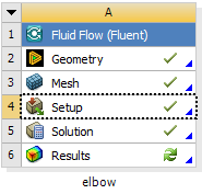
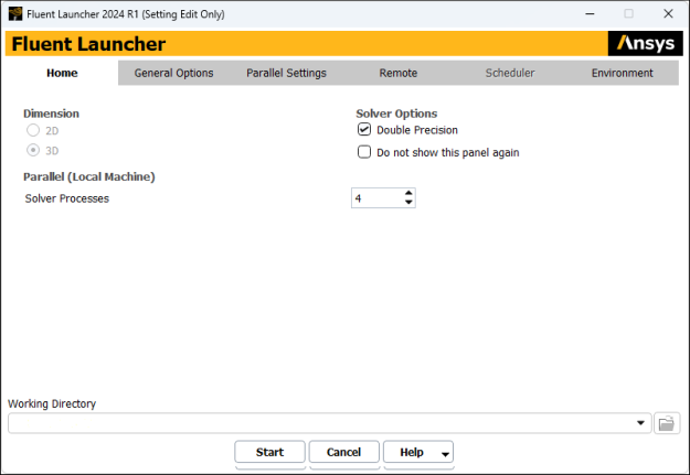
In the Ansys Workbench Project Schematic, double-click the Setup cell in the elbow fluid flow analysis system. You can also right-click the Setup cell to display the context menu where you can select the Edit... option.
When Ansys Fluent is first started, the Fluent Launcher is displayed, enabling you to view and/or set certain Ansys Fluent start-up options.
Note: The Fluent Launcher allows you to decide which version of Ansys Fluent you will use, based on your geometry and on your processing capabilities.
Figure 1.11: Ansys Fluent Launcher
Ensure that the proper options are enabled.

Important: Note that the Dimension setting is already filled in and cannot be changed, since Ansys Fluent automatically sets it based on the mesh or geometry for the current system.
1. Select Double Precision under Options.
2. Set Solver Processes to 4 under Parallel (Local Machine).
Note: Fluent will retain your preferences for future sessions.
Click Start to launch Ansys Fluent.
Note: The Ansys Fluent settings file (FFF.set) is written as soon as Ansys Fluent opens.
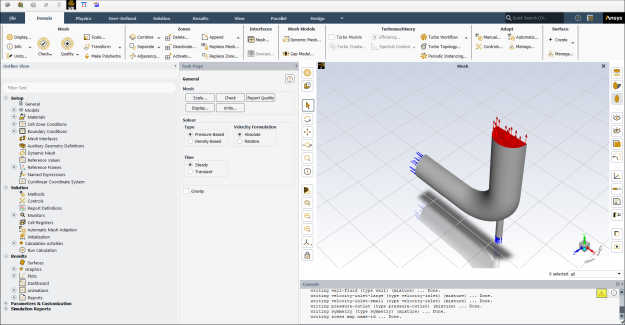
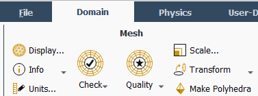
Figure 1.12: The Ansys Fluent Application

1.4.5.2. Setting Up Domain

In this step, you will perform the mesh-related activities using the Domain ribbon tab (Mesh group).

Note: These controls are also available in the General task page that can be accessed by clicking the Setup/General tree item.

Change the units for length.
Because you want to specify and view values based on a unit of length in millimeters from within Ansys Fluent, change the units of length within Ansys Fluent from meters (the default) to millimeters.

Important: Note that the Ansys Meshing application automatically converts and exports meshes for Ansys Fluent using meters (m) as the unit of length regardless of what units were used to create them. This is so you do not have to scale the mesh in Ansys Fluent under Ansys Workbench.

Domain → Mesh → Units...
This displays the Set Units dialog box.
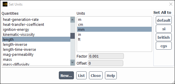
1. Select length in the Quantities list.
2. Select mm in the Units list.
3. Close the dialog box.
Note: Now, all subsequent inputs that require a value based on a unit of length can be specified in millimeters rather than meters.
Check the mesh.
Domain → Mesh → Check → Perform Mesh Check
Note: Ansys Fluent will report the results of the mesh check in the console.
```
 Domain Extents:
   x-coordinate: min (m) = -2.000000e-01, max (m) = 2.000000e-01
   y-coordinate: min (m) = -2.250000e-01, max (m) = 2.000000e-01
   z-coordinate: min (m) = 0.000000e+00, max (m) = 5.000000e-02
 Volume statistics:
   minimum volume (m3): 2.896709e-09
   maximum volume (m3): 5.870990e-08
     total volume (m3): 2.510838e-03
 Face area statistics:
   minimum face area (m2): 1.854435e-06
   maximum face area (m2): 4.386908e-05
 Checking mesh.....................................
Done.
```
Note: The minimum and maximum values may vary slightly when running on different platforms. The mesh check will list the minimum and maximum x and y values from the mesh in the default SI unit of meters. It will also report a number of other mesh features that are checked. Any errors in the mesh will be reported at this time. Ensure that the minimum volume is not negative as Ansys Fluent cannot begin a calculation when this is the case.
Review the mesh quality.
Domain → Mesh → Quality → Evaluate Mesh Quality
Note: Ansys Fluent will report the results of the mesh quality below the results of the mesh check in the console.
```
Mesh Quality:

Minimum Orthogonal Quality =  2.25949e-01 cell 27293 on zone 4 (ID: 244 on partition: 0) 
at location ( 1.25755e-01, -1.56954e-01,  3.15732e-03)

Maximum Aspect Ratio =  3.09204e+01 cell 27293 on zone 4 (ID: 244 on partition: 0) 
at location ( 1.25755e-01, -1.56954e-01,  3.15732e-03)
```
Note: The quality of the mesh plays a significant role in the accuracy and stability of the numerical computation. Checking the quality of your mesh is, therefore, an important step in performing a robust simulation. Minimum cell orthogonal quality is an important indicator of mesh quality. Values for orthogonal quality can vary between 0 and 1 with lower values indicating poorer quality cells. In general, the minimum orthogonal quality should not be below 0.01 with the average value significantly larger. The high aspect ratio cells in this mesh are near the walls and are a result of the boundary layer inflation applied in the meshing step. For more information about the importance of mesh quality refer to the Fluent User's Guide.

1.4.5.3. Setting Up Physics

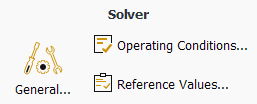
In the steps that follow, you will select a solver and specify physical models, material properties, and zone conditions for your simulation using the Setting Up Physics ribbon tab.

In the Solver group of the Physics ribbon tab, retain the default selection of the steady pressure-based solver.
Physics → Solver
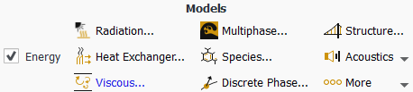
Set up your models for the CFD simulation using the Models group of the Physics ribbon tab.

Note: You can also use the Models task page that can be accessed by double-clicking the Setup/Models tree item.
1. Enable heat transfer by activating the energy equation.
  In the Physics ribbon tab, select Energy (Models group).
  Physics → Models → Energy
2. Enable the k-ω SST turbulence model.
  1. In the Physics ribbon tab, click Viscous... (Models group).
    Physics → Models → Viscous...
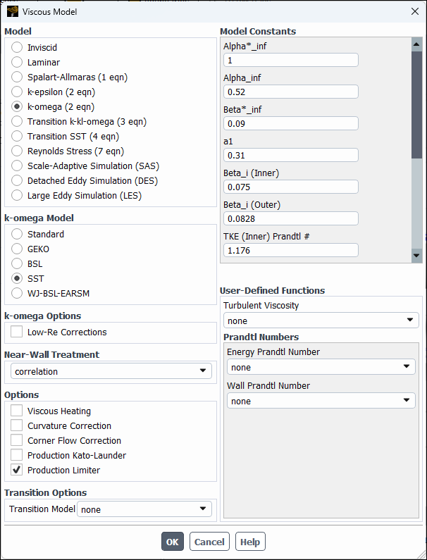
  2. In the Viscous Model dialog box, retain the default selection of k-omega from the Model list.
  3. Use the default SST from the k-omega Model group.
  4. Click OK to accept the model and close the Viscous Model dialog box.
    Note that the Viscous... label in the ribbon is displayed in blue to indicate that the Viscous model is enabled.
Set up the materials for your CFD simulation using the Materials group of the Physics ribbon tab.

Create a new material called water-liquid using the Create/Edit Materials dialog box.
1. In the Setting Up Physics ribbon tab, click Create/Edit... (Materials group).
  Physics → Materials → Create/Edit...
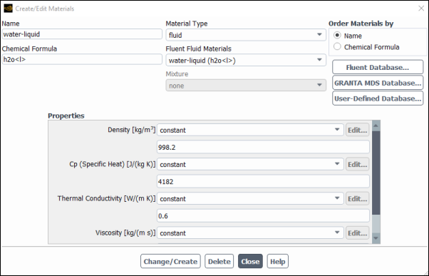
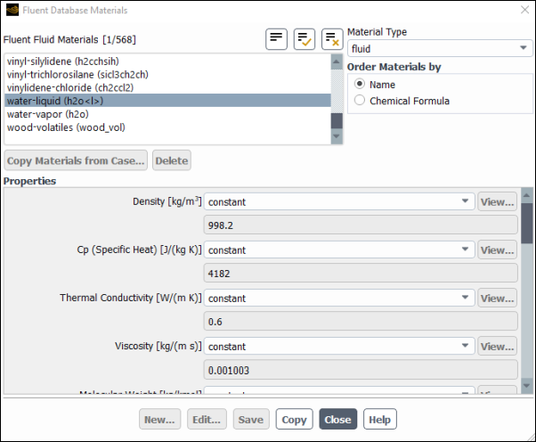
2. Copy the material water-liquid (h2o < l >) from the materials database (accessed by clicking the Fluent Database... button).
  Figure 1.13: The Create/Edit Materials Dialog Box
3. Select water-liquid (h2o < l >) from the materials list and Click Copy, then close the Fluent Database... panel.
4. Ensure that there are now two materials (water and air) defined locally by examining the Fluent Fluid Materials drop-down list in the Create/Edit Materials dialog box .
  Note: Both the materials will also be listed under Fluid in the Materials task page and under the Materials tree branch.
5. Close the Create/Edit Materials dialog box.
Set up the cell zone conditions for the CFD simulation using the Zones group of the Physics ribbon tab.
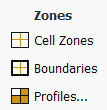
1. In the Physics tab, click Cell Zones.
  Physics → Zones → Cell Zones
  This opens the Cell Zone Conditions task page.
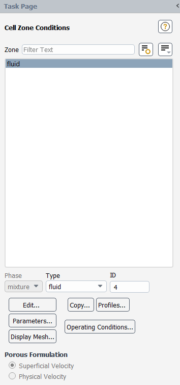
2. Set the cell zone conditions for the fluid zone.
  1. In the Cell Zone Conditions task page, in the Zone list, select fluid and click Edit... to open the Fluid dialog box.
    Note: You can also double-click fluid in the Cell Zones Conditions task page or under the Setup/Cell Zone Conditions tree branch in order to open the corresponding dialog box.
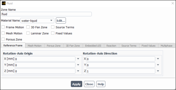
  2. Select water-liquid from the Material Name drop-down list.
  3. Click Apply and close the Fluid dialog box.

Set up the boundary conditions for the CFD analysis using the Zones group of the Physics ribbon tab.

In the Physics tab, click Boundaries (Zones group).
Physics → Zones → Boundaries
This opens the Boundary Conditions task page.

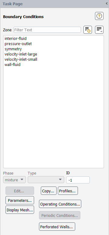
Note: To display boundary zones grouped by zone type (as shown above), click the Toggle Tree View button in the upper right corner of the Boundary Conditions task page and under the Group By category select Zone Type from the drop-down list.
Set the boundary conditions at the cold inlet (velocity-inlet-large).
Tip: If you are unsure of which inlet zone corresponds to the cold inlet, you can use the mouse to probe for mesh information in the graphics window. If you click the right mouse button with the pointer on any node in the mesh, information about the associated zone will be displayed in the Ansys Fluent console, including the name of the zone. The zone you probed will be automatically selected from the Zone selection list in the Boundary Conditions task page.
Alternatively, you can click the probe button ( ) in the graphics toolbar and click the left mouse button on any node. This feature is especially useful when you have several zones of the same type and you want to distinguish between them quickly. The information will be displayed in the console.
1. From the Zone selection list, select velocity-inlet-large and click Edit....
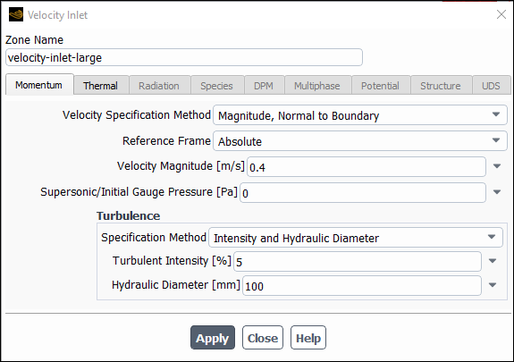
2. In the Velocity Inlet dialog box, ensure that Magnitude, Normal to Boundary is selected for Velocity Specification Method.
3. Enter 0.4 for Velocity Magnitude.
4. In the Turbulence group, from the Specification Method drop-down list, select Intensity and Hydraulic Diameter.
5. Retain the default of 5 for Turbulent Intensity.
6. Enter 100 mm for Hydraulic Diameter.
  Note: The hydraulic diameter is defined as:
  where is the cross-sectional area and is the wetted perimeter.
7. Click the Thermal tab.
8. Enter 293.15 for Temperature.
9. Click Apply and close the Velocity Inlet dialog box.

In a similar manner, set the boundary conditions at the hot inlet (velocity-inlet-small), using the values in the following table:

Setting	Value
Velocity Specification Method	Magnitude, Normal to Boundary
Velocity Magnitude	`1.2` [m/s]
Specification Method	Intensity & Hydraulic Diameter
Turbulent Intensity	`5`%
Hydraulic Diameter	`25` [mm]
Temperature	`313.15`[K]

Double-click pressure-outlet and set the boundary conditions at the outlet, as shown in the Pressure Outlet dialog box.

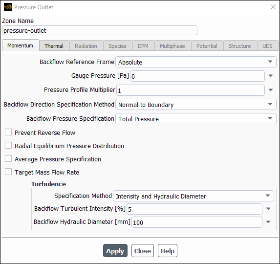
Note: Ansys Fluent will use the backflow conditions only if the fluid is flowing into the computational domain through the outlet. Since backflow might occur at some point during the solution procedure, you should set reasonable backflow conditions to prevent convergence from being adversely affected.

1.4.6. Solving

In the steps that follow, you will set up and run the calculation using the Solution ribbon tab.

Note: You can also use the task pages listed under the Solution branch in the tree to perform solution-related activities.

Set up solution parameters for the CFD simulation.
1. 1. In the Solution ribbon tab, click Methods... (Solution group).
    Solution → Solution → Methods...
    This will open the Solution Methods task page.
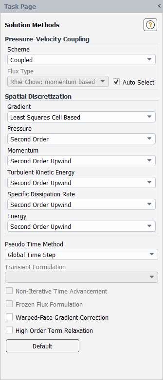
  2. Retain the default selections.
2. Enable the plotting of residuals during the calculation.
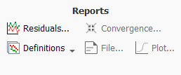
  1. In the Solution ribbon tab, click Residuals... (Reports group).
    Solution → Reports → Residuals...
    
    In the Residual Monitors dialog box, ensure that Plot is enabled in the Options group.
  2. Keep the default values for the Absolute Criteria of the Residuals, as shown in the Residual Monitors dialog box.
  3. Click OK to close the Residual Monitors dialog box.
  Note: By default, all variables will be monitored and checked by Ansys Fluent as a means to determine the convergence of the solution.
3. Create a surface report definition at the outlet (pressure-outlet).
  Solution → Reports → Definitions → New → Surface Report → Facet Maximum
  1. In the Surface Report Definition dialog box, enter temp-outlet-0 for the Name.
  2. Under the Create group, enable Report File and Report Plot.
    During a solution run, Ansys Fluent will write solution convergence data in a report file and plot the solution convergence history in a graphics window.
    It is good practice to monitor physical solution quantities in addition to equation residuals when assessing convergence.
  3. Set Frequency to 3 by clicking the up-arrow button.
    This setting instructs Ansys Fluent to update the plot of the surface report and write data to a file after every 3 iterations during the solution.
  4. Select Temperature... and Static Temperature from the Field Variable drop-down lists.
  5. Select pressure-outlet from the Surfaces selection list.
  6. Click OK to save the surface report definition and close the Surface Report Definition dialog box.
    The new surface report definition temp-outlet-0 appears under the Solution/Report Definitions tree item. Ansys Fluent also automatically creates the following items:
    temp-outlet-0-rfile (under the Solution/Monitors/Report Files tree branch)
    temp-outlet-0-rplot (under the Solution/Monitors/Report Plots tree branch)
4. In the tree, double-click the temp-outlet-0-rfile (under the Solution/Monitors/Report Files) and examine the report file settings in the Edit Report File dialog box.
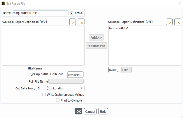
  The dialog box is automatically populated with data from the temp-outlet-0 report definition. The report that will be written in a report file during a solution is listed under Selected Report Definitions.
  Retain the default output file name and click OK.
5. In the tree, double-click temp-outlet-0-rplot (under Solution/Monitors/Report Plots) and examine the report plot settings in the Edit Report Plot dialog box.
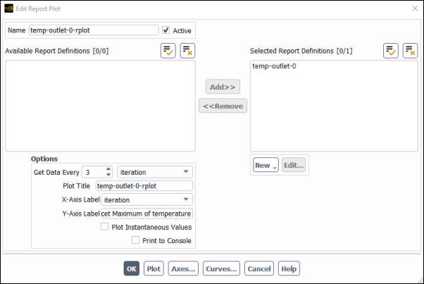
  The dialog box is automatically populated with data from the temp-outlet-0 report definition. As the solution progresses, the report that is listed under Selected Report Definitions will be plotted in a graphics tab window with the title specified in Plot Title.
  Retain the default names for Plot Title and Y-Axis Label and click OK.
  Note: You can create report definitions for different boundaries and plot them in the same graphics window. However, report definitions in the same Report Plot must have the same units.
6. Initialize the flow field using the Initialization group of the Solution ribbon tab.
  Solution → Initialization
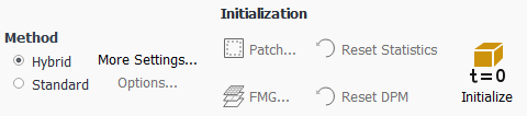
  1. Keep the Method at the default of Hybrid.
  2. Click Initialize.
Calculate a solution using the Run Calculation group of the Solution tab.
Solution → Run Calculation
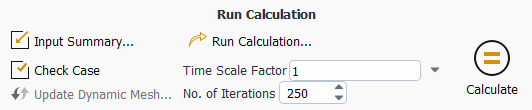
1. Start the calculation by requesting 250 iterations.
  1. Enter 250 for No. of Iterations.
  2. Click Calculate.
  Note that while the program is calculating the solution, the states of the Setup and Solution cells in the fluid flow Ansys Fluent analysis system in Ansys Workbench are changing. For example:
  - The state of the Setup cell becomes Up-to-Date and the state of the Solution cell becomes Refresh Required after the Run Calculation task page is visited and the number of iterations is specified.
  - The state of the Solution cell is Update Required while iterations are taking place.
  - The state of the Solution cell is Up-to-Date when the specified number of iterations are complete (or if convergence is reached).
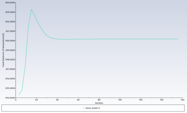
  As the calculation progresses, the surface report plot will be plotted in the graphics window (temp-outlet-0–rplot tab window) (Figure 1.14: Convergence History of the Maximum Temperature at Pressure Outlet).
  Figure 1.14: Convergence History of the Maximum Temperature at Pressure Outlet
  
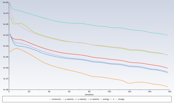
  The residuals history will be plotted in the Scaled Residuals tab window (Figure 1.15: Residuals for the Converged Solution).
  Figure 1.15: Residuals for the Converged Solution
  
  Note: The solution will be stopped by Ansys Fluent when the residuals reach their specified values or after 250 iterations. The exact number of iterations will vary depending on the platform being used. An Information dialog box will open to alert you that the calculation is complete. Click OK in the Information dialog box to proceed.
  Because the residual values vary slightly by platform, the plot that appears on your screen may not be exactly the same as the one shown here.
  Note that the Ansys Fluent settings file (FFF.set) is updated in the Files view of the Ansys Workbench before the calculation begins.
2. Examine the plots for convergence (Figure 1.15: Residuals for the Converged Solution and Figure 1.14: Convergence History of the Maximum Temperature at Pressure Outlet).
  Note: There are no universal metrics for judging convergence. Residual definitions that are useful for one class of problem are sometimes misleading for other classes of problems. Therefore it is a good idea to judge convergence not only by examining residual levels, but also by monitoring relevant integrated quantities and checking for mass and energy balances.
  There are three indicators that convergence has been reached:
  The residuals have decreased to a sufficient degree.
  The solution has converged when the Convergence Criterion for each variable has been reached. The default criterion is that each residual will be reduced to a value of less than , except the energy residual, for which the default criterion is .
  The solution no longer changes with more iterations.
  Sometimes the residuals may not fall below the convergence criterion set in the case setup. However, monitoring the representative flow variables through iterations may show that the residuals have stagnated and do not change with further iterations. This could also be considered as convergence.
  The overall mass, momentum, energy, and scalar balances are obtained.
  You can examine the overall mass, momentum, energy and scalar balances in the Flux Reports dialog box. The net imbalance should be less than 0.2 of the net flux through the domain when the solution has converged. In the next step you will check to see if the mass balance indicates convergence.
With Ansys Fluent still running, go back to Ansys Workbench and view the list of generated files.
View → Files
Note the addition of the surface report definition file temp-outlet-0.out to the list of files.
The status of the Solution cell is now up-to-date.

1.4.7. Displaying Results in Ansys Fluent and CFD-Post

In this step, you will display the results of the simulation in Ansys Fluent, display the results in CFD-Post, and then review the list of files generated by Ansys Workbench.

Display results in Ansys Fluent using the Results ribbon tab.
In Ansys Fluent, you can perform a simple evaluation of the velocity and temperature contours on the symmetry plane. Later, you will use CFD-Post (from within Ansys Workbench) to perform the same evaluation.
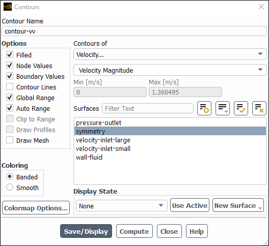
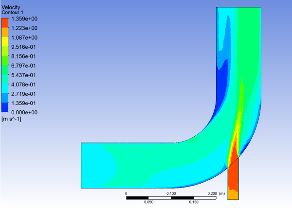
1. Display filled contours of velocity magnitude on the symmetry plane (Figure 1.16: Velocity Distribution Along Symmetry Plane).
  Results → Graphics → Contours → New...
  Note: You can also double-click the Results/Graphics/Contours tree item.
  1. Enter contour-vv for Contour Name.
  2. In the Contours dialog box, in the Options group, enable Filled.
  3. Select Banded in the Coloring group box.
  4. Ensure that Node Values and Boundary Values is enabled in the Options group.
  5. From the Contours of drop-down lists, select Velocity... and Velocity Magnitude.
  6. From the Surfaces selection list, deselect all items by clicking and then select symmetry.
  7. Click Display to display the contours in the active graphics window.
  Figure 1.16: Velocity Distribution Along Symmetry Plane
  
  Note: You may want to clear Headlight and Lighting in the Viewing ribbon tab (Display group).
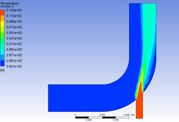
2. Display filled contours of temperature on the symmetry plane (Figure 1.17: Temperature Distribution Along Symmetry Plane).
  Results → Graphics → Contours → New...
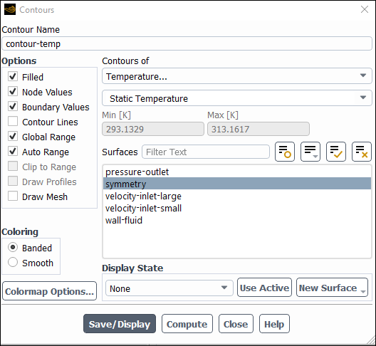
  1. Enter contour-temp for Contour Name.
  2. Select Banded in the Coloring group box.
  3. Select Temperature... and Static Temperature from the Contours of drop-down lists.
  4. Click Display and close the Contours dialog box.
  Figure 1.17: Temperature Distribution Along Symmetry Plane
3. Close the Ansys Fluent application.
  File → Close Fluent
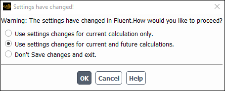
  Important: Note that the Ansys Fluent case and data files are automatically saved when you exit Ansys Fluent and return to Ansys Workbench.
  The following prompt is presented, whenever settings change in Ansys Fluent and in the Project Schematic the Solution cell might need to be refreshed..
4. View the list of files generated by Ansys Workbench.
  View → Files
  Note the addition of the compressed Ansys Fluent case and data files to the list of files. These will have names like FFF-1.cas.gz and FFF-1-00167.dat.gz. Note that the digit(s) following FFF may be different if you have had to restart the meshing or calculation steps for any reason and that the name of the data file is based on the number of iterations. Thus your file names may be slightly different than those shown here.
Display results in CFD-Post.
1. Start CFD-Post.
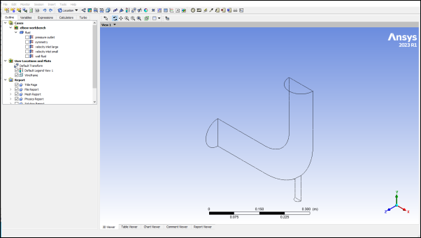
  In the Ansys Workbench Project Schematic, double-click the Results cell in the elbow fluid flow analysis system (cell A6). This displays the CFD-Post application. You can also right-click the Results cell to display the context menu where you can select the Edit... option.
  Note: The elbow geometry is already loaded and is displayed in outline mode. Ansys Fluent case and data files are also automatically loaded into CFD-Post.
  Figure 1.18: The Elbow Geometry Loaded into CFD-Post
2. Reorient the display.
  Click the blue Z axis on the axis triad in the bottom right hand corner of the graphics display to orient the display so that the view is of the front of the elbow geometry.
3. Ensure that Highlighting ( ) is disabled.
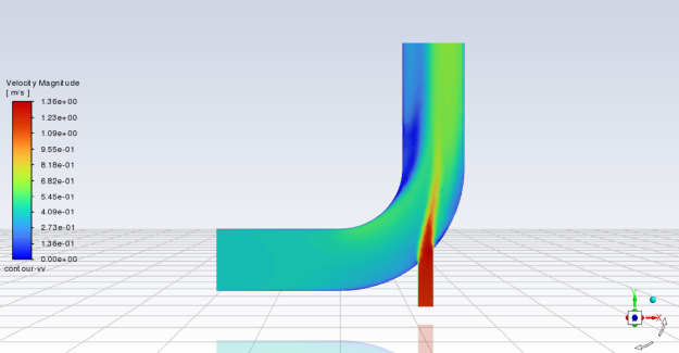
4. Display contours of velocity magnitude on the symmetry plane (Figure 1.19: Velocity Distribution Along Symmetry Plane).
  1. Insert a contour object using the Insert menu item at the top of the CFD-Post window.
    Insert → Contour
    This displays the Insert Contour dialog box.
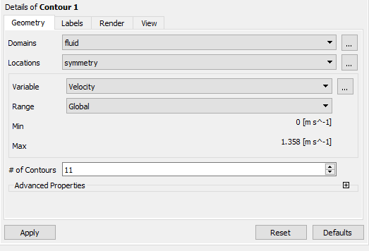
  2. Keep the default name of the contour (Contour 1) and click OK to close the dialog box. This displays the Details of Contour 1 view below the Outline view in CFD-Post. This view contains all of the settings for a contour object.
  3. In the Geometry tab, from the Domains drop-down list, select fluid.
  4. In the Locations list, select symmetry.
  5. In the Variable list, select Velocity.
  6. Click Apply.
  Figure 1.19: Velocity Distribution Along Symmetry Plane
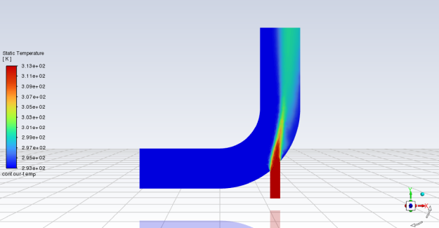
5. Display contours of temperature on the symmetry plane (Figure 1.20: Temperature Distribution Along Symmetry Plane).
  1. In the Outline tree view, under User Locations and Plots, clear the check box beside the Contour 1 object to disable the Contour 1 object and hide the first contour display.
  2. Insert a contour object.
    Insert → Contour
    This displays the Insert Contour dialog box.
  3. Keep the default name of the contour (Contour 2) and click OK to close the dialog box. This displays the Details of Contour 2 view below the Outline view.
  4. In the Geometry tab, from the Domains drop-down list, select fluid.
  5. In the Locations list, select symmetry.
  6. In the Variable list, select Temperature.
  7. Click Apply.
  Figure 1.20: Temperature Distribution Along Symmetry Plane
Close the CFD-Post application by selecting File → Close CFD-Post or by clicking the ‘X’ in the top right corner of the window.

Important: Note that the CFD-Post state files are automatically saved when you exit CFD-Post and return to Ansys Workbench.
Save the elbow-workbench project in Ansys Workbench.
View the list of files generated by Ansys Workbench.
View → Files
Note the addition of the CFD-Post state file (elbow.cst) to the list of files. For more information about CFD-Post (and the files associated with it), see the CFD-Post documentation.

1.4.8. Duplicating the Fluent-Based Fluid Flow Analysis System

At this point, you have a completely defined fluid flow system that has a geometry, a computational mesh, a CFD setup and solution, and corresponding results. In order to study the effects upon the flow field that may occur if you were to alter the geometry, another fluid flow analysis is required. One approach would be to use the current system and change the geometry, however you would overwrite the data from your previous simulation. A more suitable and effective approach would be to create a copy, or duplicate, of the current system, and then make the appropriate changes to the duplicate system.

In this step, you will create a duplicate of the original Fluent-based fluid flow system, then review the list of files generated by Ansys Workbench.

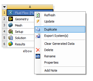
In the Project Schematic, right-click the title cell of the Fluid Flow (Fluent) system and select Duplicate from the context menu.
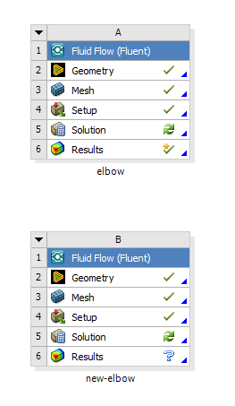
Figure 1.21: Duplicating the Fluid Flow System

Figure 1.22: The Original Fluid Flow System and Its Duplicate

Note: Notice that in the duplicated system, the state of the Solution cell indicates that the cell requires a refresh while the state of the Results cell indicates that the cell requires attention. This is because when a system is duplicated, the case and data files are not copied to the new system, therefore, the new system does not yet have solution data associated with it.
Rename the duplicated system to new-elbow.
Save the elbow-workbench project in Ansys Workbench.

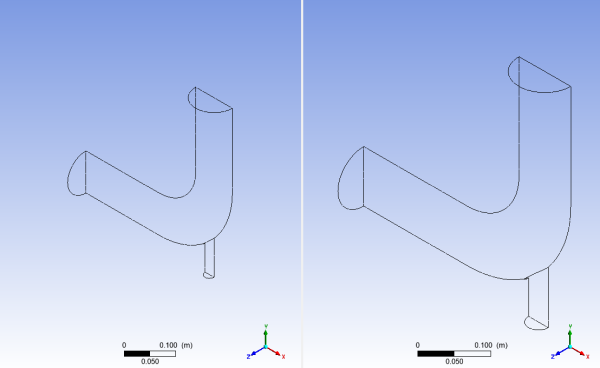
1.4.9. Changing the Geometry in Ansys DesignModeler

Now that you have two separate, but equivalent, Fluent-based fluid flow systems to work from, you can make changes to the second system without impacting the original system. In this step, you will make a slight alteration to the elbow geometry in Ansys DesignModeler by changing the diameter of the smaller inlet, then review the list of files generated by Ansys Workbench.

Open Ansys DesignModeler.
Right-click the Geometry cell of the new-elbow system (cell B2) and select Edit Geometry in DesignModeler... from the context menu to display the geometry in Ansys DesignModeler.
Change the diameter of the small inlet (velocity-inlet-small).
1. In the Tree Outline, select Cylinder1 to open the Details View of the small inlet pipe.
2. In the Details View, change the FD10, Radius (>0) value from 12.5 millimeters to 19 millimeters.
3. Click the Generate button to generate the geometry with your new values.
  Figure 1.23: Changing the Diameter of the Small Inlet in Ansys DesignModeler
Close Ansys DesignModeler.
View the list of files generated by Ansys Workbench.
View → Files
Note the addition of the geometry, mesh, and Ansys Fluent settings files now associated with the new, duplicated system.

1.4.10. Updating the Mesh in the Ansys Meshing Application

The modified geometry now requires a new computational mesh. The mesh settings for the duplicated system are retained in the duplicated system. In this step, you will update the mesh based on the mesh settings from the original system, then review the list of files generated by Ansys Workbench.

In the Project Schematic, right-click the Mesh cell of the new-elbow system (cell B3) and select Update from the context menu. This will update the mesh for the new geometry based on the mesh settings you specified earlier in the Ansys Meshing application without having to open the Ansys Meshing editor to regenerate the mesh.

It will take a few moments to update the mesh. Once the update is complete, the state of the Mesh cell is changed to up-to-date, symbolized by a green check mark.

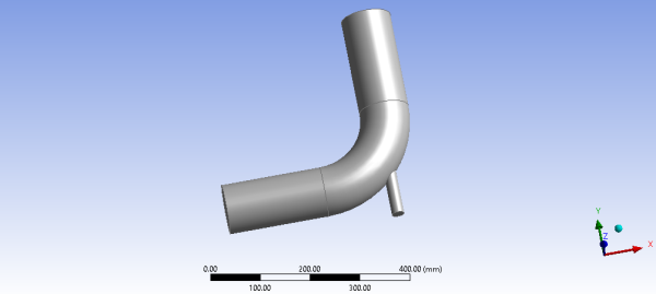
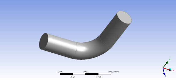
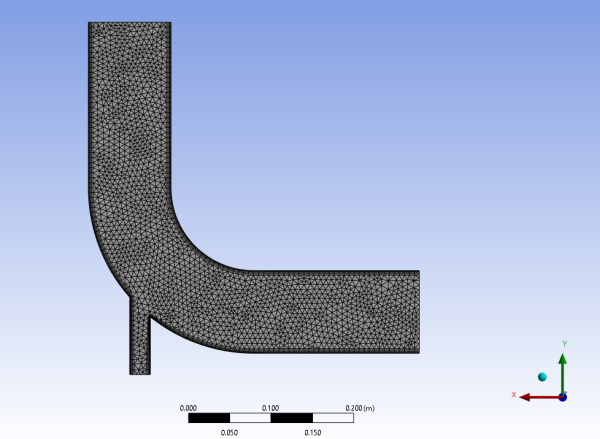
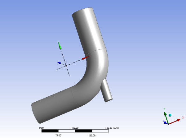
For illustrative purposes of the tutorial, the new geometry and the new mesh are displayed below.

Figure 1.24: The Updated Geometry and Mesh in the Ansys Meshing Application

Inspecting the files generated by Ansys Workbench reveals the updated mesh file for the duplicated system.

View → Files

1.4.11. Calculating a New Solution in Ansys Fluent

Now that there is an updated computational mesh for the modified geometry in the duplicated system, a new solution must be generated using Ansys Fluent. In this step, you will revisit the settings within Ansys Fluent, calculate another solution, view the new results, then review the list of files generated by Ansys Workbench.

Open Ansys Fluent.
In the Project Schematic, right-click the Setup cell of the new-elbow system (cell B4) and select Edit... from the context menu. Since the mesh has been changed, you are prompted as to whether you want to load the new mesh into Ansys Fluent or not.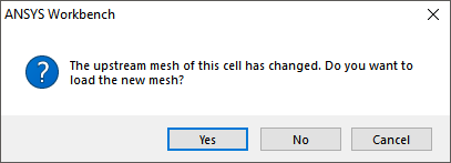
Click Yes to continue, and click Start when Fluent Launcher is displayed in order to open Ansys Fluent.
Ensure that the unit of length is set to millimeters.
Domain → Mesh → Units...
Check the mesh (optional).
Setting Up Domain → Mesh → Check → Perform Mesh Check
Revisit the boundary conditions for the small inlet.
Setup → Boundary Conditions → velocity-inlet-small Edit...
In the Velocity Inlet dialog box for velocity-inlet-small, you must set the hydraulic diameter to 38 mm based on the new dimensions of the small inlet.
Re-initialize the solution.
Solution → Initialization
Keep the Method at the default of Hybrid and click Initialize.
Recalculate the solution.
Solution → Run Calculation → Calculate
Set the No. of Iterations to 250 and click Calculate.
Close Ansys Fluent.
Revisit the results of the calculations in CFD-Post.
Double-click the Results cell of the new-elbow fluid flow system to re-open CFD-Post where you can review the results of the new solution.
Close CFD-Post.
Save the elbow-workbench project in Ansys Workbench.
View the list of files generated by Ansys Workbench.
View → Files
Note the addition of the solution and state files now associated with new duplicated system.

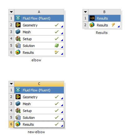
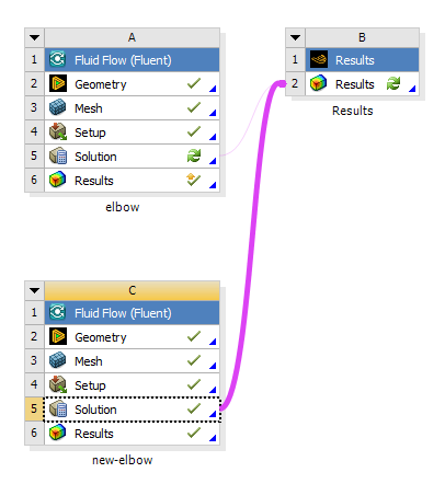
1.4.12. Comparing the Results of Both Systems in CFD-Post

In this step, you will create a new Results system in Ansys Workbench, use that system to compare the solutions from each of the two Fluent-based fluid flow analysis systems in CFD-Post at the same time, then review the list of files generated by Ansys Workbench.

Create a Results system.
In Ansys Workbench, drag a Results system from the Component Systems section of the Toolbox and drop it into the Project Schematic, next to the fluid flow systems.
Figure 1.25: The New Results System in the Project Schematic
Add the solutions of each of the systems to the Results system.
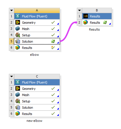
1. Select the Solution cell in the first Fluid Flow analysis system (cell A5) and drag it over the Results cell in the Results system (cell B2). This creates a transfer data connection between the two systems.
  Figure 1.26: Connecting the First Fluid Flow System to the New Results System
2. Select the Solution cell in the second Fluid Flow analysis system (cell C5) and drag it over the Results cell in the Results system (cell B2). This creates a transfer data connection between the two systems.
  Figure 1.27: Connecting the Second Fluid Flow System to the New Results System
Open CFD-Post to compare the results of the two fluid flow systems.
Now that the two fluid flow systems are connected to the Results system, double-click the Results cell in the Results system (cell C2) to open CFD-Post. Within CFD-Post, both geometries are displayed side by side.
Figure 1.28: CFD-Post with Both Fluid Flow Systems Displayed
1. Re-orient the display.
  In each view, click the blue Z axis on the axis triad in the bottom right hand corner of the graphics display to orient the display so that the view is of the front of the elbow geometry.
  
  Important: Alternatively, you can select the synchronization tool ( ) in the 3D Viewer Toolbar to synchronize the views, so that when you re-orient one view, the other view is automatically updated.
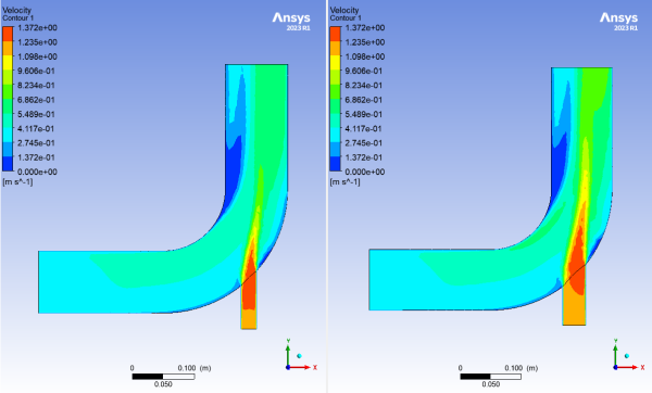
2. Display contours of velocity magnitude on the symmetry plane.
  1. Insert a contour object.
    Insert → Contour
    This displays the Insert Contour dialog box.
  2. Keep the default name of the contour (Contour 1) and click OK to close the dialog box. This displays the Details of Contour 1 view below the Outline view in CFD-Post. This view contains all of the settings for a contour object.
  3. In the Geometry tab, from the Domains list, select fluid.
  4. In the Locations list, select symmetry.
  5. In the Variable list, select Velocity.
  6. Click Apply. The velocity contours are displayed in each view.
  Note: To better visualize the velocity display, you can clear the Wireframe view option under User Locations and Plots in the Outline tree view.
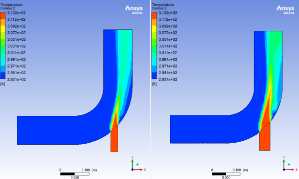
  Figure 1.29: CFD-Post Displaying Velocity Contours for Both Geometries
3. Display contours of temperature on the symmetry plane.
  1. In the Outline tree view, under User Locations and Plots, deselect the Contour 1 object to hide the first contour display in CFD-Post.
  2. Insert another contour object.
    Insert → Contour
    This displays the Insert Contour dialog box.
  3. Keep the default name of the contour (Contour 2) and click OK to close the dialog box. This displays the Details of Contour 2 view below the Outline view in CFD-Post.
  4. In the Geometry tab, select fluid in the Domains list.
  5. Select symmetry in the Locations list.
  6. Select Temperature in the Variable list.
  7. Click Apply. The temperature contours are displayed in each view.
  Figure 1.30: CFD-Post Displaying Temperature Contours for Both Geometries
Close the CFD-Post application.
Save the elbow-workbench project in Ansys Workbench.
View the list of files associated with your project using the Files view.
View → Files
Note the addition of the Results system and its corresponding files.

1.5. Summary

In this tutorial, portions of Ansys Workbench were used to compare the fluid flow through two slightly different geometries. Ansys DesignModeler was used to create a mixing elbow geometry, Ansys Meshing was used to create a computational mesh, Ansys Fluent was used to calculate the fluid flow throughout the geometry using the computational mesh, and CFD-Post was used to analyze the results. In addition, the geometry was altered, a new mesh was generated, and a new solution was calculated. Finally, Ansys Workbench was set up so that CFD-Post could directly compare the results of both calculations at the same time.