


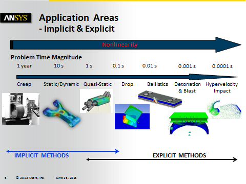
Implicit and Explicit finite element solvers use different methods to evaluate the underlying equations. A simple high level overview is given in the figure below. There is an overlap in the "Quasi-Static" application area, where both Implicit and Explicit methods can be used to solve a model. Implicit methods are typically bounded by the amount of deformation and contact nonlinearity that is taking place, where Explicit methods are typically bounded by the problem's time scale, which would lead to excessive run times.
Problems that are in this "Quasi-Static" range have a good chance of being solved by either method until the limitations of a particular solver are reached. At that point, it can be beneficial to consider the use of the alternative solver.
This chapter describes the steps necessary to transform a model that was initially set up for simulation in the Implicit solver to a model setup for simulation in the Explicit solver. Typically, you would want to consider doing this when the degree of nonlinearity in the model is starting to pose problems for Implicit methods. Because of the nature of the two methods, the explicit solver is more suitable for nonlinear problems, working with less computationally heavy but a much larger number of iterations that can follow the physical parameter changes at a much higher frequency. The implicit solver works with much more complex calculations for each iteration but has a lot fewer of them.