


This model is used for modeling brittle materials such as glass and ceramics (Johnson & Holmquist 1993) [1] subjected to large pressures, shear strain and high strain rates. Two forms of this model are found in the literature and are available in explicit dynamics systems; continuous (JH2), segmented (JH1).
Both these forms can be used with a linear or energy dependent polynomial equation of state.
The strength of the brittle material is described as a smoothly varying function
of intact strength, fractured strength, strain rate and damage via a dimensionless
analytic function as described below. P* is the pressure normalized by the pressure
at the Hugoniot Elastic Limit (PHELL) and T* is the maximum
tensile hydrostatic pressure normalized by PHELL. The
effective plastic strain rate,  , is normalized by a reference strain rate of 1.0/second.
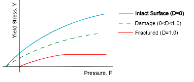
Intact Surface, 
Damage, 
Fractured, 
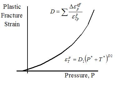
As the material undergoes inelastic deformation, damage is assumed to accumulate which degrades the overall load carrying capacity of the materials. The Johnson-Holmquist Damage model was developed for the simulation of the compressive and shear induced strength and failure of brittle materials. Damage is accumulated as the ratio of incremental plastic strain over the current estimated fracture strain. The effective fracture strain is pressure dependent as described below.
There are two methods for the application of damage to the material strength. The default Gradual failure type results in damage being incrementally applied to the material strength as it accumulates. If the Instantaneous failure type is selected, damage accumulates over time, however it is only applied to the failure surface when its value reaches unity. The material strength instantaneously transitions from intact to fully failed in this case.
The model includes an option to represent volumetric dilation of the material due to shear deformation (Bulking). The work done in deforming the material inelastically in shear can be converted into a pressure increase, hence volumetric dilation (if unconstrained). The amount of work which is converted into dilation pressure is controlled through the Bulking constant, B. This can have values ranging from 0.0 (representing no shear induced dilatancy) to 1.0 (producing maximum dilatancy effects).
Note: If the Bulking constant, B is greater than zero then the Johnson-Holmquist model should be used in conjunction with a polynomial equation of state or linear elasticity.
This property can only be applied to solid bodies.
Table 11.7: Input Data
| Name | Symbol | Units | Notes |
|---|---|---|---|
| Hugoniot Elastic Limit | σHEL | Stress | Elastic limit under dynamic compressive uniaxial strain conditions |
| Intact Strength Constant A | A | None | |
| Intact Strength Exponent n | n | None | |
| Strain Rate Constant C | C | None | |
| Fracture Strength Constant B | B | None | |
| Fracture Strength Exponent m | m | None | |
| Maximum Fracture Strength Ratio | σF Max | None | Maximum fracture strength as fraction of intact strength |
| Damage Constant D1 | D1 | None | |
| Damage Constant D2 | D2 | None | |
| Bulking Constant | B | None | |
| Hydrodynamic Tensile Limit | T | Stress | |
| Failure Type | Option list: Gradual (Default) Instantaneous |
Custom results variables available for this model:
| Name | Description | Solids | Shells | Beams |
|---|---|---|---|---|
| EFF_Pl_STN | Effective Plastic Strain | Yes | No | No |
| EFF_Pl_STN_RATE | Effective Plastic Strain Rate | Yes | No | No |
| PRESSURE | Pressure | Yes | No | No |
| DAMAGE | Damage | Yes | No | No |
| STATUS | Material Status** | Yes | No | No |
| PRES_BULK | Dilation pressure | Yes | No | No |
| ENERGY_DAM | Damage energy contributing to bulking | Yes | No | No |
**Material status indicators (1= elastic, 2= plastic, 3 = bulk failure, 4 = bulk failure, 5 = failed principal direction 1, 6 = failed principal direction 2, 7 = failed direction 3)