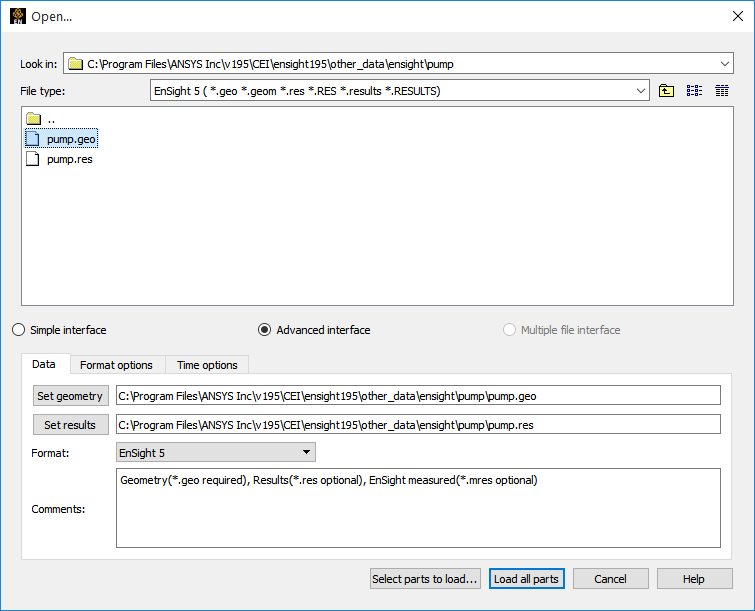
Measured data is read into EnSight naturally via the casefile (for EnSight6 and EnSight Gold formats) or can be read with other mesh formats via the Format options tab in the Open... dialog, as shown below:
Select → to open the dialog for data file selection.
Find the directory containing the data (see Read Data for more information on using File Selection).
Click .
In the Data tab, select and set the needed information for the (meshed) geometry, including the Format, geometry file, and if applicable, the result file.
Open the Format options tab and select and set the measured result file.
Now you can continue the normal process of either , or
See Read Data for more information on using File Selection.
Measured data is represented as a single part. In the main Parts list you should see a part named Measured/Particle after loading.
Measured data is represented as a set of unconnected nodes. You can use EnSight's ability to display nodes in various ways to accentuate measured data visualization. To change node display:
Select the desired measured data part in the Parts list.
Click the Node representation icon.

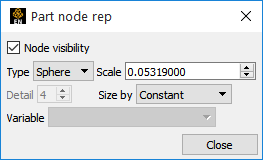
Which opens the Part Node Rep dialog. Node visibility will be on by default for measured data parts.
Select the desired node display type
Dot: nodes are displayed as points.
Cross: nodes are displayed as crosses and can be fixed sized (size set by the Scale value) or sized based on a Variable (and scaled by the Scale value).
Sphere: nodes are displayed as spheres and can be fixed sized (size set by the Scale value) or sized based on a Variable (and scaled by the Scale value). Sphere detail controlled by Detail value.
: particles in an SPH point part are treated as spheres and a surface is extracted on the fly using a screen space voxel grid rendered into an outer surface.
If applicable, set desired values for Scale, Detail, Size By, and Variable.
Smoothed-particle hydrodynamics (SPH) is a meshless approach for simulating the mechanics of continuum media, such as solid mechanics and fluid flows. Given the 0D discrete solution result for SPH solutions, there is desire to display this given 0D discrete solution as a continuum, or more importantly, visually as some type of fluid-like continuous surface (from the collection of discrete solution points).
The screen space surface rendering technique is a method utilized by EnSight to efficiently render those discrete locations in the client’s screen space as a pseudo continuous fluid-like surface. The technique effectively renders each discrete point as a sphere of a specified size, until these spheres begin to overlap sufficiently, and then are rendered as a more continuous surface. This technique blurs the line between a discrete simulation and the artistic representation of a continuous surface. Currently, there are three major factors which influence the visualization technique: represented sphere size, spatial resolution of the discrete SPH solution location, and the effective number of neighbors that each particle has.
Sphere Size
You can start off by utilizing an SPH_Radius variable exported by your solver, and start with a scaling factor of
2.0(this will represent the particle as their physical size). The scale factor may need to be adjusted up or down from here to suit the desired rendering result. If you do not have an SPH_Radius variable, then using a constant scale factor setting, and adjusting the value of the scale from a small number upwards to the desired overlap will be required.Spatial Resolution
The SPH screen space rendering technique relies upon the overlap of particles to generate the surface of interest. Therefore, solutions with sparse spatial resolution will need to use a larger scale factor for the sphere size to obtain sufficient overlap to create the look of a continuous surface.
Note: In this case, it might be more realistic to rerun the solution with more particles.
Number of Neighbors
The third aspect influencing the combination of discrete locations into a continuous surface is the effective number of neighbors for each SPH location. If the number of neighbors is small, then you should not be making these artificially too large (creating larger droplets of fluid which were not meant by the SPH solver routine).
The main factor (sphere size) will be required for all SPH rendering solutions. Depending upon your exact solution, you may be able to stop here. However, adjustment of the sphere size depending upon your spatial resolution may be required. Utilization of the number of neighbors may also need to be utilized in situations where the solution contains both small and large collection of droplets.
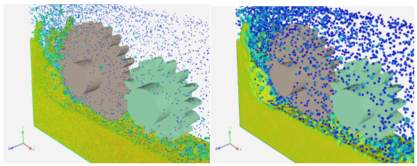
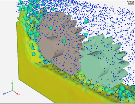
In the example above, using SPH_Radius and a scale factor of
2(right) yields good main fluid volume rendering, but the droplets are too large and overpower the rendering. Using a scale factor smaller than2(left) yields a good droplet size, but the main fluid volume is not rendered as a continuous region.In this example, the color refers to the number of neighbors. Utilization of the number of neighbors is needed to generate a better visualization. There are a few different techniques at your disposal for utilizing the number of neighbors variable.
Binary Filter
You can utilize Filter elements
 , with a binary
threshold to completely ignore particles with number of neighbors less than the value
specified.
, with a binary
threshold to completely ignore particles with number of neighbors less than the value
specified.Note: In this case, any particle with a number of neighbors less than 8 is entirely ignored.
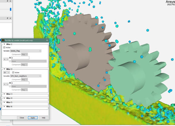
This removes the particle entirely from the solution (not just visually). Take this into account when performing quantitative analysis or conveying results to the audience.
Multiple IsoVolumes
You can use the feature in EnSight,
 Isosurfaces → , to break up the single
SPH part into multiple SPH parts based on their number of neighbors (There are currently three
parts: 0 to 3; 3 to 11, 12 and higher). With three parts, you can change the scale factor for
each part to size each grouping accordingly (small neighbor counts have a small scale factor,
large neighbor counts have a larger scale factor).
Isosurfaces → , to break up the single
SPH part into multiple SPH parts based on their number of neighbors (There are currently three
parts: 0 to 3; 3 to 11, 12 and higher). With three parts, you can change the scale factor for
each part to size each grouping accordingly (small neighbor counts have a small scale factor,
large neighbor counts have a larger scale factor).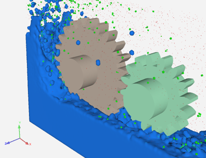
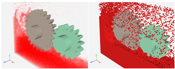
The small neighbor count SPH particles (red) are set to a small scale factor (
0.25); the medium neighbor counts (green) are set to a moderate scale factor (1.0), and the large neighbor counts (blue) are set to a larger scale factor (3.0).Calculator Function
A third option to employ the number of neighbors is with a calculator function. In this case, you write a single function, comprised of a series of greater than & less than operations to allow you to retain the single original SPH part, while using a scale factor which takes into account number of neighbors.

This results in the following rendering.
Your results using can be greatly improved by experimenting with these various techniques to control and specify the size of the spheres. This allows you to obtain an appropriate rendering to convey the visual representation desired. The values and specifics will vary based on your model, solution, and other factors. This is an area which is rather artistic, and there is significantly more user-specific interpretation involved in the setup of this rendering technique.