


EnSight’s default operation with Transient models and variables may be different to your Fluent operation. With Transient models in EnSight, when you first activate a variable (either through coloration or part creation based on it), EnSight takes the variable’s extrema at that timestep to determine the current range of the palette used for that variable. If you change timesteps, the range is not automatically changed (by default), and therefore the coloration stays consistent between timestep changes, but the range in the palette may not reflect the current range of the variable in the model.
There are a few options in EnSight to cater to the changes in variable range over time.
Option 1
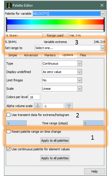
Automatically adjust the palette on timestep change (each timestep the min/max of the palette is changed to match the current timestep’s min/max). Simply toggle on the option in the Palette editor.
Option 2
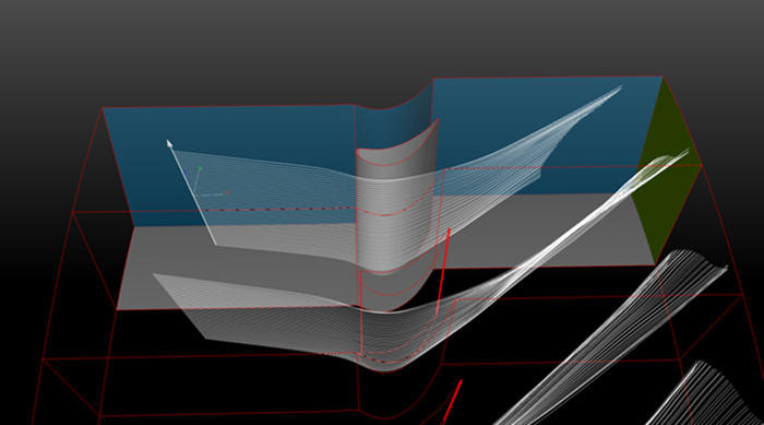
You can turn on the to instruct EnSight to use the temporal min/max to determine the Set Range to in location (3) in the image below.
EnSight has a fully featured calculator to determine new spatial, temporal derived variables from a relatively wide set of both PreDefined functions (for example Spatial Mean, or Flow Rates) or user defined equations (for example Cp = Pressure / Pdyn). In addition, you can calculate can derived quantities from the solution based on either nodal or elemental based variables (variables defined at nodes/vertices or elements/cells). Data read in through the Fluent .cas/.dat file reader into EnSight is elemental based, while data exported from Fluent to the EnSight Case format can be either nodal or elemental. EnSight can also convert from nodal to/from elemental data using a very basic straight averaging routine. As Fluent’s solver is elemental based, if you desire to calculate elemental based variables (for example Volume Weighted Average Temperature) as close to that reported by Fluent, you should utilize elemental variables exported from Fluent, or directly through the .cas/.dat reader. The differences in variable calculation between nodal and elemental variables differ only in regions which suffer from high gradients relative to the discretization used.
The Calculator feature of EnSight contains a few predefined variables that can be used to calculate mass weighted averages.
The first function is SpaMeanWeighted(). This function takes as input two variables, and returns the sum of variable1 * variable2 * the size of the elements divided by the sum of variable2 * the size of the elements. So, it returns the average of variable1 weighted by variable2. If you set variable2 to be the density, this is the same as the mass-weighted average.
Note: This function works both on 2D and 3D elements (the only difference being, you'll need to use surface or volumetric density).
Fluent contains two functions that calculate Mass-Weighted Averages. From the Fluent documentation:
Surface Integral of Mass-Weighted Average
The mass-weighted average of a quantity is computed by dividing the summation of the value of the selected field variable multiplied by the absolute value of the dot product of the facet area and momentum vectors by the summation of the absolute value of the dot product of the facet area and momentum vectors (surface mass flux)
EnSight's calculator function MassFluxAvg is the equivalent of this Fluent function.
Note: This definition includes velocity and Normal vector fields (which isn't the case for the next function).
Volume Integral of Mass-Weighted Average
The mass-weighted average of a quantity is computed by dividing the summation of the product of density, cell volume, and the selected field variable by the summation of the product of density and cell volume.
EnSight's SpaMeanWeighted() function with volumetric density as the second variable is equivalent to this function.
EnSight has a comprehensive Calculator to perform not only new spatial (for example Pressure / 0.5 * rho * velocity2) or temporal variables (for example TemporalMean), the calculator can be used to calculate items like Flow rate (Flow() function), Line/Surface/Volume integrals, boundary layer calculations, min distance calculations, element metrics, and many more. Reference the Ansys EnSight User Manual chapter on Calculator (Calculator) to obtain a broader picture of the capabilities within EnSight to derive analytical quantities from the domain and variables.
Note: This note is written as of EnSight version 10.2.2(b).
In Fluent, you can visualize the values of variables on these symmetry planes. When you then bring the data into EnSight, some variables appear to be undefined on these symmetry planes.
Why Does This Happen?
The post processor contained in Fluent has information about the physics of the simulation, and how this physics is implemented in the solver. It knows that this is a symmetry part, and therefore when you ask to visualize a variable on it, it knows how to take the values from the fluid domain and extract them correctly onto the symmetry plane part. On the other hand, EnSight has no knowledge about the settings of the simulation. For some variables, the data files that Fluent exports do not contain their values on the part that corresponds to the symmetry plane, and EnSight doesn't know that this is a symmetry plane, and it doesn't know how to correctly extract the values from the fluid domain onto this part. Therefore, it leaves these variables as undefined.
Is There a Work-Around?
If you are reading Exported data from Fluent to EnSight Case format
YES. If you utilize the Fluent export to EnSight format, you will receive variable values on boundaries like symmetry planes.
If you are reading Fluent .cas/.dat files
Unfortunately, there isn't any work around. The data simply isn't contained in the files EnSight has access to, and EnSight cannot do the physical interpolations needed to derive these values. One possibility is to use the calculator CaseMap function to map onto the symmetry plane the value of the variables just inside the fluid.
A modification to the fluent reader is planned to attempt to address this issue of missing/non existent variable values on certain boundaries (symmetry planes being one of them).
Note: This isn't an extrapolation but simply a copy-paste of the values from the fluid onto the symmetry part, so it will still show a slight difference compared to the results in Fluent.
As a part of the simulation set up in Fluent, you can set some parts to be Boundaries, fixing the value of a variable on them. When doing so, if you create a Contour for the Boundary part in Fluent with this variable, you will know exactly what values will be visualized.
If now you bring the data into EnSight and colors the Boundary part by the variable, it's possible that you will not see the expected value.
What Is Going On?
Fluent stores the information about the variable values at the elements centroid, usually. On a Boundary part, though, the value that is imposed by you is stored at the nodes. The element centroid will contain a value that is the interpolation between the faces on the Boundary part and the neighboring fluid elements - so, a value that will not correspond with what you have set as Boundary condition.
When you ask Fluent for a contour of the Boundary part, Fluent knows that this is a Boundary and therefore, instead of showing the value of the variable at the element centroid, as it would usually do, it shows the values at the nodes.
EnSight doesn't have access to the same level of knowledge. When you ask to visualize a variable on a part, EnSight doesn't know if the part is a Boundary part or not, and will simply show what the data file contains. So, if the data file contains the variable stored at the elements centroid, this is what is going to be visualized - which will look incorrect to you and not consistent with what Fluent displays.
You can verify that, indeed, the data is the same in the two software by toggling off the in Fluent (which will force it to display the elemental values), or by using the Fluent console to extract the values at the Boundary.
Introduction
Introduced in EnSight 10.2, is the ability to generate Periodic Streamlines. This allows models which were solved using Periodic Boundaries (sometimes referred to as Cyclic Boundaries) to create streamlines which re-enter the domain when the streamline exits through one of the periodic face. The re-enter point is the corresponding location on the matching periodic face. This can be quite helpful in visualizing a complete streamline, rather than the streamline stopping when it has reached the physical extent of the domain (rather than the computational extent of the domain). This capability exists for both Streamlines (steady state) and Pathlines (transient).
Procedure
There are two basic items which need to be setup for calculating Periodic Streamlines.
The parent of the streamline (typically the fluid part(s)) must have their periodicity setup within the Part Visual Symmetry dialog box.
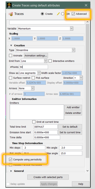
When creating the streamline, you must have the Compute Using Periodicity option turned ON.
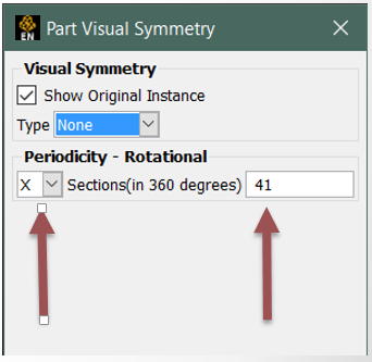
The Parent of the streamline (typically the fluid part(s)) must have their periodicity setup. For each parent part, Visual Symmetry must be setup for the appropriate rotational periodicity.
The Axis of Periodicity must be set.
The number of Sections in a full 360 degrees must be set.
The creation of the streamline must have the toggle enabled. This toggle can be found in the section of the Create Traces using default attributes dialog:
Note:Most solvers apply this periodicity as a face boundary condition. However, in EnSight, the specification of periodicity is done to the fluid domain, and NOT to the periodic face. In the example below, both the orange and blue parts need to be specified as periodic for streamlines to correctly pass through. If you fail to specify the blue part as periodic, the streamlines can appear to stop at the interface.

As the streamline exits the physical domain of the parents, the parents are checked for their periodicity, and if on, EnSight then looks at the periodic copy for existence of a domain and continues to integrate the streamline. The visual presentation of the periodic streamline remains within the physical boundaries of the parent part.
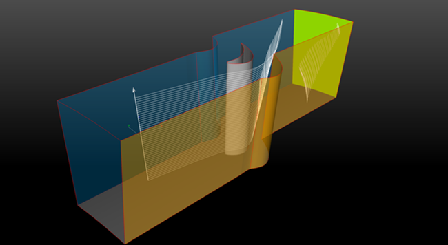
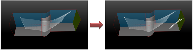
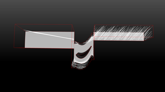
Passages can have different periodic (angular) extents. Each different periodic (angular) extent should be a different part, so that you can specify the appropriate periodicity sector count for each angular extent. In the example below, there are at least 3 fluid parts, allowing 3 different angular repeat sectors. You can see that this single rake of streamlines can be correctly computed through the different angular passages, which in this case, results in what appears to be many streamlines in the downstream portion (due to high swirl).
To visualize more than the one passage of streamlines, you must do the following two steps:
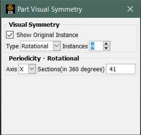
Fluid Parent: Turn on the Rotational symmetry and Instances in the Part Visual Symmetry dialog
Streamline Part: Toggle on the in the Part Visual Symmetry dialog.
For the Fluid Parents, the dialog would look like:
For the Streamline Part, the dialog would look like:
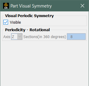
The reason why you only have a visible toggle in the Streamline's Part Visual Symmetry dialog is that the streamline may pass through different angular extents, requiring differing amounts of rotational offset along its path. Therefore, it does not make sense to have a single angular setting for the streamline. Instead, EnSight determines the angular setting based on which parent it currently is contained.
In the end, you can visualize a continuous streamline from inlet to outlet by visualizing more than a single instance:
For a generic example to try yourself, you will find below a link to an EnSight session file containing an example dataset.
Download the
Periodic_Streamline_Example_Setup.zipfile here .You have a single .ens file. Simply load this into EnSight. For setup, you will need to know that the periodicity angular sector count is 41 (there are 41 sections in 360 degrees) about the X-axis. You should be able to follow the above instructions to try out periodic streamlines.
Caveats
Does not work with Massed Traces
Does not work with Surface Restricted Traces.
Only works in Rotationally Periodic models.