


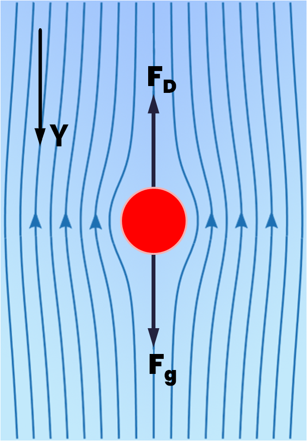
In this verification case, a spherical particle freely falls under both the gravitational force and a separate drag force due to a prescribed vertical airflow. The particle accelerates due to gravity and gradually decelerates due to the fluid's drag force, reaching a constant velocity referred to as the terminal velocity when the drag force is equal to the gravitational force.
The falling sphere schematics with acting forces and vertical flow streamlines are shown in Figure 3.1: Particle falling under gravitational and drag forces.. For more imformation about how CFD models and methods are implemented in Rocky, refer to the Rocky DEM-CFD Coupling Technical Manual.
The drag force,  , acting on the particle is calculated based upon the drag coefficient
 [4]:
[4]:
 | (3–1) |
where:
 is the relative velocity between the particle and fluid.
  is the projected particle area in the flow direction.
  is the fluid density.
Considering that the sphere shown in is a sufficiently small particle of diameter
 , its velocity
  can be evaluated from the following expression:
 | (3–2) |
with initial conditions  and
and  , where y is the particle displacement and
 is the particle material density.
The drag coefficient  in the current example is calculated using the Schiller & Naumann
correlation, valid for
in the current example is calculated using the Schiller & Naumann
correlation, valid for  with spherical particles. For more information about the theory, refer to
the Rocky DEM-CFD Coupling Technical Manual.
with spherical particles. For more information about the theory, refer to
the Rocky DEM-CFD Coupling Technical Manual.
The equations shown in the last section can be resolved and equivalent results can be calculated by Rocky with the CFD coupling methods considering the same input data and boundary conditions. The input parameters for this verification case setup that are common for all the coupling methods used are presented in Table 3.1: Verification case input parameters..
Table 3.1: Verification case input parameters.
|
Parameter |
Value |
Unit |
|---|---|---|
|
Physical Model: | ||
| Gravity Y | -9.81 |  |
|
Solid Properties (Particle): | ||
| Shape | Sphere | - |
| Diameter | 100 |  |
| Material Density | 2000 |  |
| Initial Velocity | 0 |  |
|
Fluid Properties (1-Way Constant): | ||
| Density | 1.225 |  |
| Viscosity |  |  |
| Velocity | 0.4 |  |
| Drag Law | Schiller & Naumann | - |
| Virtual Mass Law | Disabled | - |
| Turbulent Dispersion | Disbaled | - |
| Bouyancy | Enabled | - |
|
Solver Parameters: | ||
| Simulation Duration | 0.5 |  |
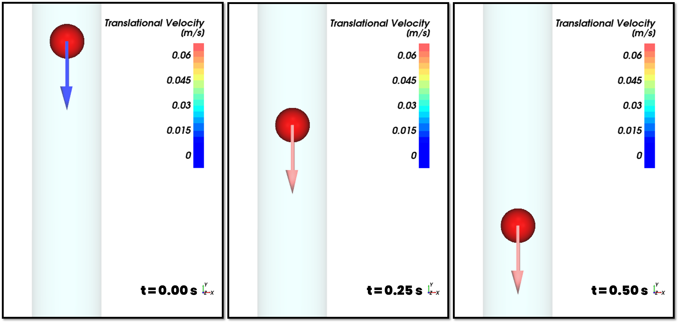
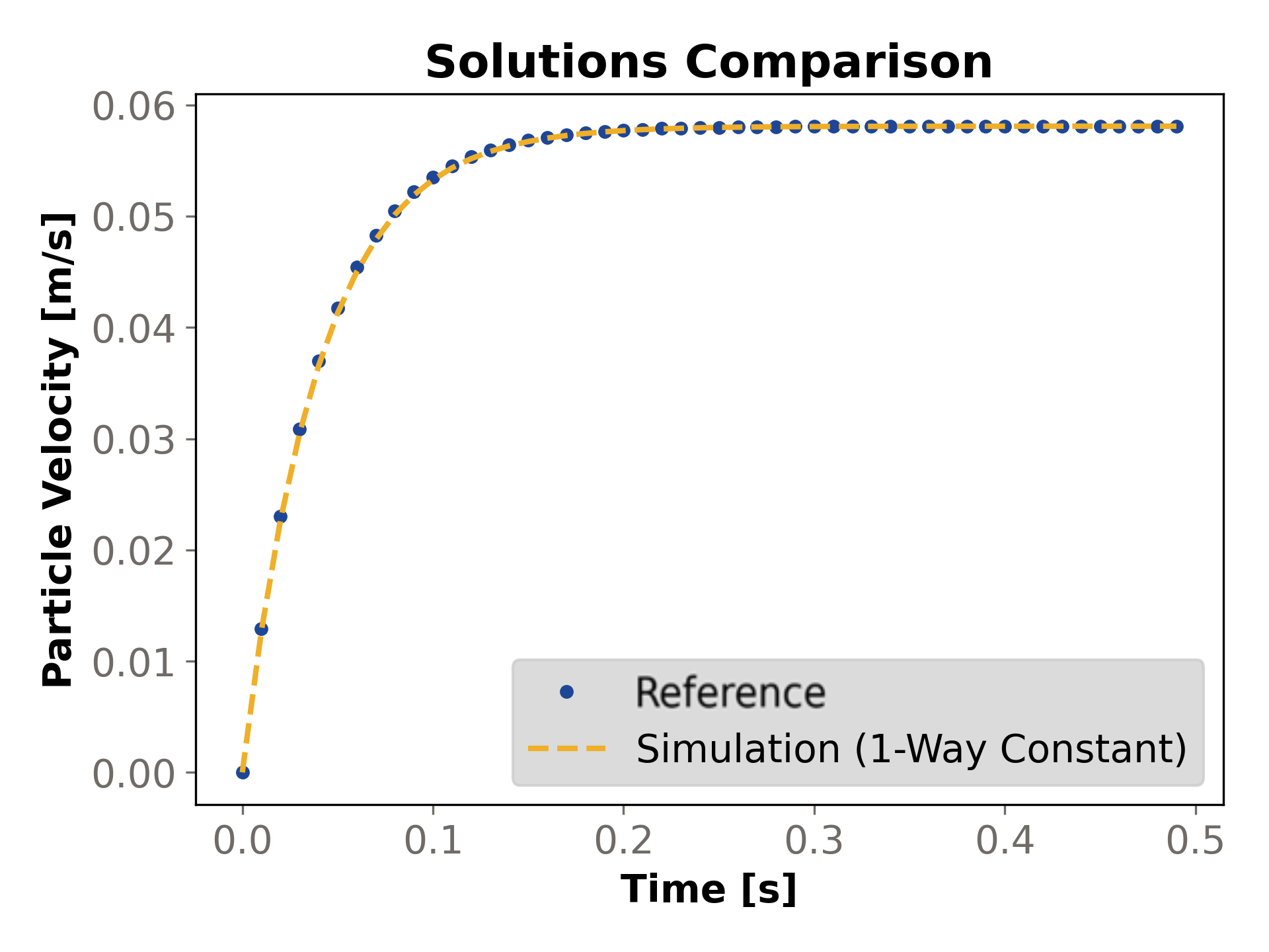
The first coupling method used was the 1-Way Constant method. When comparing the results, the particle velocity calculated by Rocky presents strongly correlated values to those obtained by the mathematical expression (named as reference). Figure 3.2: Rocky simulation results using 1-Way Constant coupling at several different output times. shows the particle velocity calculated by Rocky at three different output times. The comparison of the particle's velocity evolution over time is shown in Figure 3.3: Particle velocity over time results comparison using 1-Way Constant coupling method..
After running the Rocky case as specified, the results can then be compared to the analytical values. Figure 3.2: Rocky simulation results using 1-Way Constant coupling at several different output times. shows the particle velocity calculated by Rocky at the three different timesteps. The evolution of the particle velocity over time is shown in Figure 3.2: Rocky simulation results using 1-Way Constant coupling at several different output times.. The numerical solution given by Rocky presents strongly correlated values to those obtained by the mathematical expression.
Figure 3.2: Rocky simulation results using 1-Way Constant coupling at several different output times.
The absolute and relative errors for the particle velocity are compared in Figure 3.4: Particle velocity over time results comparison using 1-Way Constant coupling method.. The maximum absolute error for the velocity is less than 10-3 m/s. The maximum relative error is around 1.8 %.
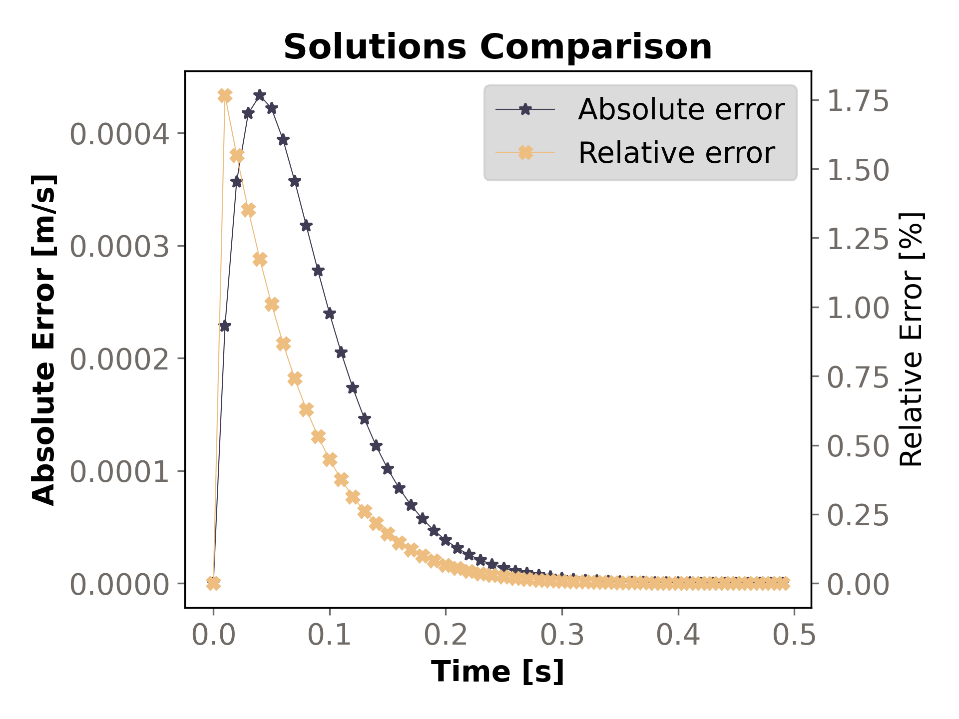
Table 3.2: Velocity target lists the value for the terminal velocity. This includes the target value calculated by the mathematical expression as compared to the value calculated by Rocky. A Ratio of 1.00000 shows a strong correlation between the results.
The second coupling method used was the 1-Way Fluent method. Similarly to the results found with the 1-Way Constant coupling method, the particle velocity calculated by Rocky presents strongly correlated values to those obtained by the mathematical expression. The comparison of the particle's velocity evolution over time is shown in Figure 3.5: Particle velocity over time results comparison using 1-Way Fluent coupling method..
After running the Rocky case as specified, the results can then be compared to the reference values. The numerical solution given by Rocky presents strongly correlated values to those obtained by the mathematical expression.
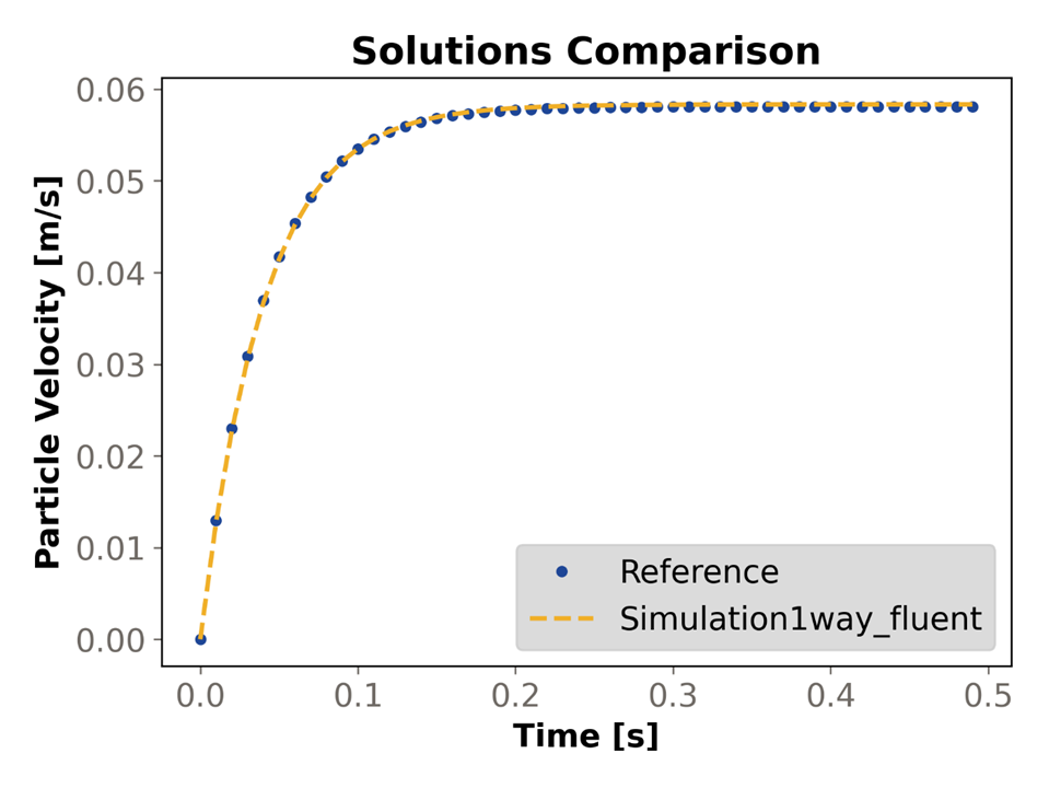
The absolute and relative errors for the particle velocity are compared in Figure 3.6: Particle velocity over time results comparison using 1-Way Fluent coupling method.. The maximum absolute error for the velocity is less than 10-3 m/s. The maximum relative error is around 1.3%.
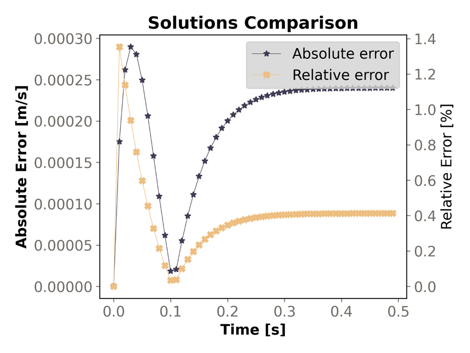
Table 3.2: Velocity target lists the value for the terminal velocity. This includes the target value calculated by the mathematical expression as compared to the value calculated by Rocky. A Ratio of 1.00430 shows a strong correlation between the results.
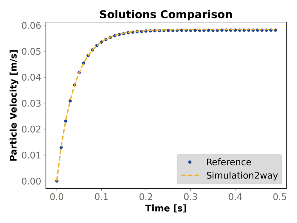
The third coupling method used was the 2-Way Unresolved method. An additional setting for the 2-Way Unresolved coupling is the Solids Maximum Volume Fraction Target, which is a reference of the space that the particles are expected to occupy within the cells of Fluent's mesh (for additional details, please check the Rocky DEM-CFD Coupling Technical Manual). This value was set to 0.0005, since the case has a single, small particle. Similarly to the results found with both coupling methods shown before, the particle velocity calculated by Rocky presents strongly correlated values to those obtained by the mathematical expression. The comparison of the particle's velocity evolution over time is shown in Figure 3.7: Particle velocity over time results comparison using 2-Way Unresolved coupling method..
After running the Rocky case as specified, the results can then be compared to the reference values. The numerical solution given by Rocky presents strongly correlated values to those obtained by the mathematical expression.
The absolute and relative errors for the particle velocity are compared in Figure 3.8: Particle velocity over time results comparison using 2-Way Unresolved coupling method.. The maximum absolute error for the velocity is less than 10-3 m/s. The maximum relative error is around 1.6%.
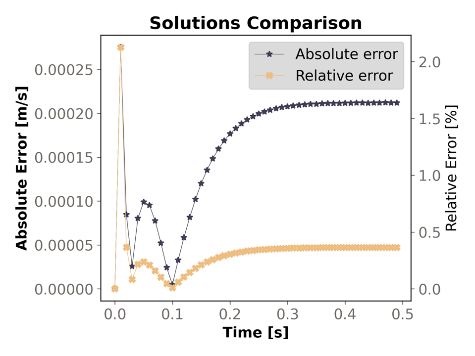
Table 3.2: Velocity target list the value for the terminal velocity. This includes the target value calculated by the mathematical expression as compared to the value calculated by Rocky. A Ratio of 1.00379 shows a strong correlation between the results.