


Broadly speaking, contact detection comprehends all geometrical calculations related to the interaction among particles and between particles and boundaries. Geometrical data needed for the calculation of contact forces is computed during the contact detection phase. Since Rocky deals with several types of particle shapes, including custom polyhedral shapes of arbitrary complexity, contact detection can easily take up a significant percentage of the total processing time.
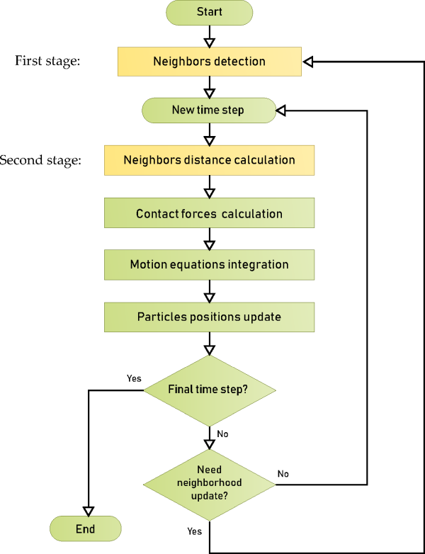
In order to optimize processing time, contact detection operations are performed in two independent stages, as indicated in the flowchart shown in Figure 5.1: Contact detection stages in the general algorithm in Rocky.. The first stage is a rough search that aims to determine a list of the particles that are closest to every particle in the simulation. Since this is a costly operation, it is performed only after some number of simulation timesteps, as indicated in the referred flowchart. In the second stage, which is performed in every timestep, the exact distances between neighbor particles are computed. In fact, all relevant geometrical information regarding every pair of neighbor particle-particle or neighbor particle-boundary is calculated in this stage, taking into account the most recent positions of the particles in the simulation.
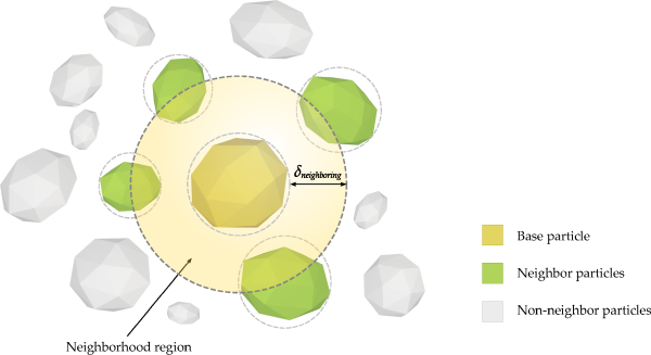
In Rocky, neighbors of a particle are all particles located at a distance less than a
predetermined value, herein called neighboring distance. This is
illustrated schematically in Figure 5.2: Neighborhood region of a particle in Rocky.. The actual geometry of the particles is
not taken into account in the first stage of neighbor detection. Since this operation must
involve every pair of particles in the simulation, considering their actual geometry would be
infeasible. Instead, in order to determine if a particle is in the neighborhood region of
another, bounding spheres are considered around every particle. Therefore, a particle will be
included into the list of neighbors of another if the distance between their bounding spheres
is less than  .
.
In the second stage of contact detection, neighbor pairs of particle-particle or particle-boundary are examined in detail for determining the relevant geometric parameters needed in the physical contact models. Here, the actual geometries of the particles are considered, therefore, the complexity of the calculations will depend on the type of particles employed in the simulation. By far, the simplest case is the contact between spherical particles. On the other hand, contact calculations between polyhedral particles, as those depicted in Figure 5.3: Exact distance calculation between neighbor particles., are more difficult, since multiple scenarios must be examined. For instance, the contact between polyhedra might be vertex-to-vertex, vertex-to-edge, vertex-to-face, edge-to-edge, edge-to-face, or even face-to-face. An extra level of complexity is added when the particles are concave, since in this case multiple contacts can arise between the same pair of particles.
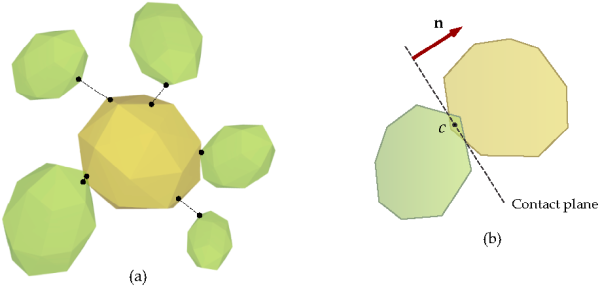
Regardless of the actual complexity of the algorithms, the end result is the set of all relevant geometrical parameters associated to a contact, such as the distance between particles, the application point of the contact forces, the orientation of the normal to the contact, etc. Physical contact will arise whenever the calculated distance between two particles or between a particle and a boundary is negative. The distance in this case is the normal overlap, needed for the calculation of the normal contact force.
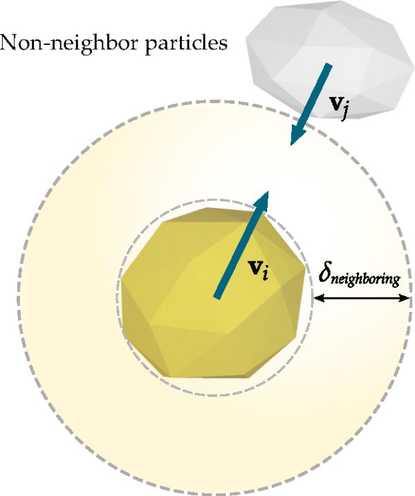
After some number of timesteps, the list of neighbors for all particles in the simulation
must be updated. Otherwise, some collisions between non-neighbor particles could arise and the
simulation would not be able to detect them. Therefore, as illustrated in Figure 5.4: Before updating neighbor lists, the maximum distance that any pair of non-neighbor
particles can move relative to each other is  ., in order to prevent missing collisions, the maximum distance that any pair of non-neighbor
particles can move relative to each other is
., in order to prevent missing collisions, the maximum distance that any pair of non-neighbor
particles can move relative to each other is  , the neighboring distance. Whenever that distance is reached, the lists of
neighbors of all particles in the simulation must be updated. Since the computation of the
exact distance can be expensive, a simplified approximate upper bound is computed in Rocky,
which guarantees that no collision will be missed in the simulations.
, the neighboring distance. Whenever that distance is reached, the lists of
neighbors of all particles in the simulation must be updated. Since the computation of the
exact distance can be expensive, a simplified approximate upper bound is computed in Rocky,
which guarantees that no collision will be missed in the simulations.
Figure 5.4: Before updating neighbor lists, the maximum distance that any pair of non-neighbor
particles can move relative to each other is .
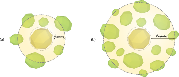
The neighboring distance  plays an important role on the performance of the contact detection
algorithms in Rocky. Figure 5.5: Two cases with different magnitude of the neighboring distance
plays an important role on the performance of the contact detection
algorithms in Rocky. Figure 5.5: Two cases with different magnitude of the neighboring distance  illustrates two opposite cases regarding the
magnitude of
illustrates two opposite cases regarding the
magnitude of  . In the first case, when the neighboring distance is low, the size of the
neighbors lists will be small and, therefore, the processing time in the second stage of
detection will be also low. This is because only a few pairs of particles will need to be
processed. However, this situation will demand more frequent updates of the neighbor lists,
and, consequently the total processing time of the first stage of contact detection may be
high. On the other hand, in the situation depicted in Figure 5.5: Two cases with different magnitude of the neighboring distance (b), when the value
of
. In the first case, when the neighboring distance is low, the size of the
neighbors lists will be small and, therefore, the processing time in the second stage of
detection will be also low. This is because only a few pairs of particles will need to be
processed. However, this situation will demand more frequent updates of the neighbor lists,
and, consequently the total processing time of the first stage of contact detection may be
high. On the other hand, in the situation depicted in Figure 5.5: Two cases with different magnitude of the neighboring distance (b), when the value
of  is relatively large, the opposite behavior is usually observed. In this
case, the elevation in the number of neighbors per particle will produce a significant
increase in the processing time of the second stage. But, at the same time, less frequent
updates of the neighbor lists will be needed, therefore, the amount of processing time of the
first stage will decrease.
is relatively large, the opposite behavior is usually observed. In this
case, the elevation in the number of neighbors per particle will produce a significant
increase in the processing time of the second stage. But, at the same time, less frequent
updates of the neighbor lists will be needed, therefore, the amount of processing time of the
first stage will decrease.
Users can override the default value of  determined internally in Rocky. This parameter can be specified in the
Advanced sub-tab of the Solver panel, where it is
listed as Neighboring Distance. As
determined internally in Rocky. This parameter can be specified in the
Advanced sub-tab of the Solver panel, where it is
listed as Neighboring Distance. As  can have a huge impact on the total processing time of a simulation, users
must be very careful when specifying its value.
can have a huge impact on the total processing time of a simulation, users
must be very careful when specifying its value.