


This script computes a steady-state flow on a contact network between a potential difference, which is specified using custom geometries bounded by a user process shape. This outcome can be useful for static bed scenarios where you want to calculate equivalent properties for the entire contact network. This script is designed to be run after the simulation is processed.
This script has specific project setup requirements that must be met before the script is run. (See the Script prerequisites section below for a detailed list.)
Script Details
Once run, the script enables you to define all of the following options:
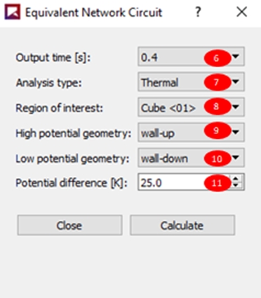
Output time [s]: Defines the output time (in seconds) for which you want the steady-state calculation to be made.
Analysis type: Defines what kind of transfer will be accounted for. (Currently, only Thermal analysis is supported.)
Region of interest: Defines the bounds of the contacts that you want to use within the contact network, the shape of which is specified through a User Process (Cube, Cylinder, or Polyhedron (Envelope)) that you create from the Contacts entity.
High potential geometry: Enables you to select which wall within your simulation has the highest potential. For thermal analysis, this means the geometry with the highest temperature.
Low potential geometry: Enables you to select which custom (imported) geometry within your simulation has the lowest potential. For thermal analysis, this means the geometry with the lowest temperature.
Potential difference [K]: Defines the temperature potential difference between the high potential geometry and the low potential geometry.
To define the bounds of the contact network upon which the steady-state flow is based, do the following:
Ensure your project setup meets all the script requirements, including:
Includes at least two walls between which the contact network will be defined.
Has only single-element (rigid) particle shapes defined.
Has the Collect Contacts Data option enabled.
Process your simulation.
Using the Time toolbar, take note of the output time (in seconds) for which you want make the calculation.
Create a User Process (Cube, Cylinder or Polyhedron (Envelope)) from the Contacts entity to be used in the script as the region of interest. The contacts encompassed within this region will form the contact network circuit.
Run the script.
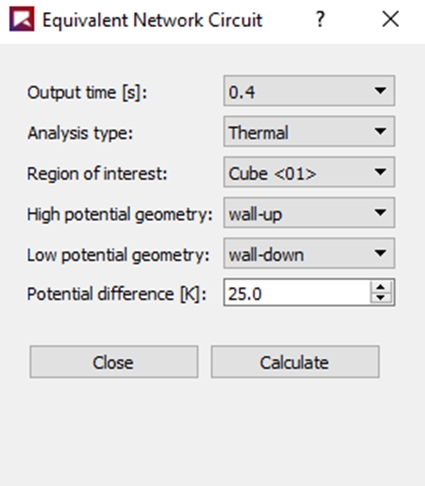
A new Equivalent Network Circuit window appears (Figure 1).
From the Output time drop-down list (figure below), select the output time for which you want make the calculation.
From the Analysis type drop-down list, select which analysis you want to do. (Currently only Thermal is supported.)
From the Region of interest drop-down list, select which User Process shape will be used as the region of interest.
From the High potential geometry drop-down list, select which wall has the highest potential.
From the Low potential geometry drop-down list, select which wall has the lowest potential.
From the Potential difference box, define the temperature potential difference between the high and low potential geometries.
Click Calculate.
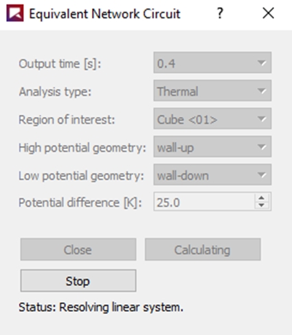
After you click Calculate, the script will resolve a linear system created within the bounds of the contact network you defined. Depending upon the number of particles, the calculation might take a few minutes to complete.
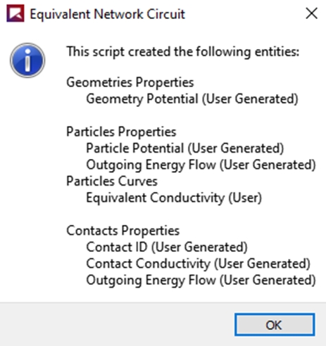
When the calculation completes, a new dialog will appear that lists the new properties and curves that are available for the affected geometry components, Particles, and Contacts entities.
Click OK to close the confirmation dialog.
Click Close on the Equivalent Network Circuit window to return to your Rocky project.
This script will create the following properties and curves:
Note: All results are based upon the Output time you defined in the script.
Individual geometry component (Property):
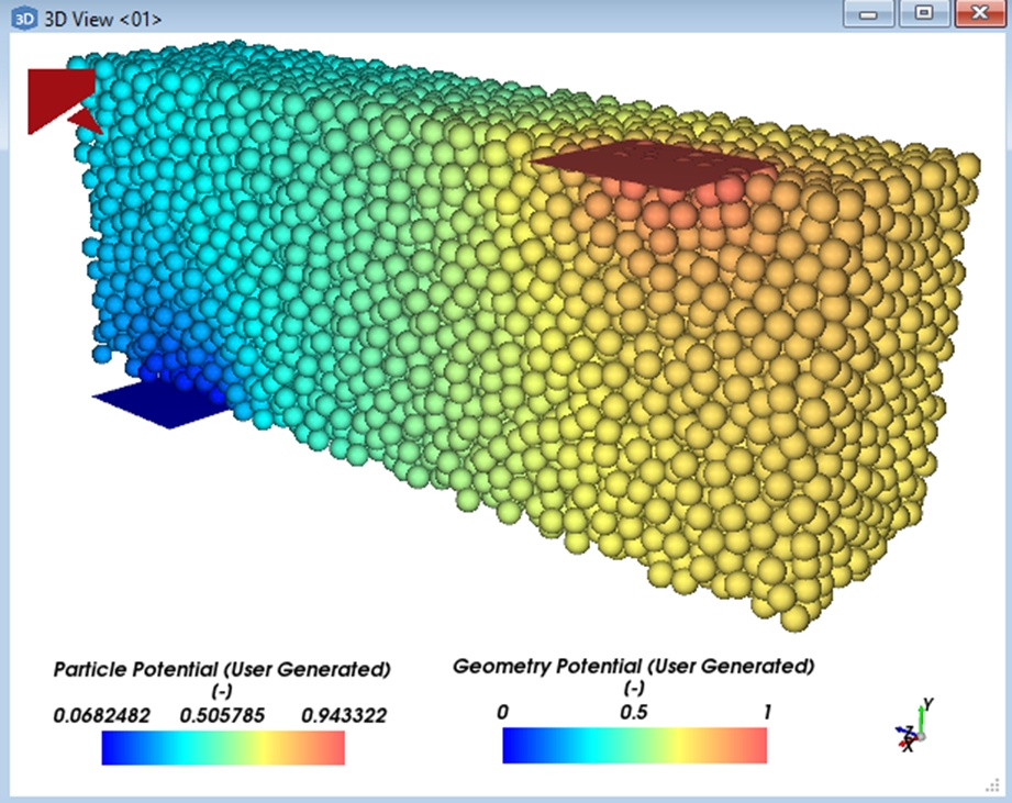
Geometry Potential (User Generated): This provides the potential of each individual whole geometry triangle. This can help you to visualize the potential of each of your geometries at the selected output time.
Particles entity (Property):
Particle Potential (User Generated): This provides the potential of each individual whole particle. This can help you to visualize the potential of each of your particles at the selected output time.
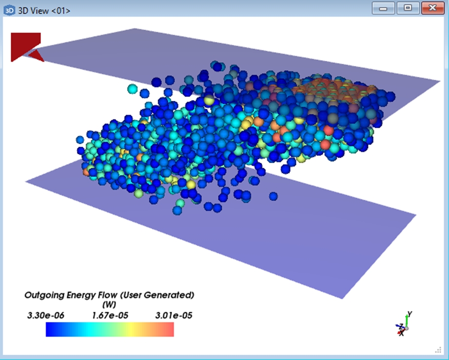
Outgoing Energy Flow (User Generated): This provides the outgoing energy flow of each individual whole particle. This can help you to visualize the amount of energy that flows on each of your particles at the selected output time.
Particles entity (Curve):
Equivalent Conductivity (User): This provides the equivalent conductivity of the entire contacts network at the selected output time.
Contacts entity (Property):
Contact ID (User Generated): This provides the ID of each individual contact.
Contact Conductivity (User Generated): This provides the conductivity of each individual contact. This can help you to visualize the conductivity on each of your contacts at the select output time.
Outgoing Energy Flow (User Generated): This provides the outgoing energy flow of each individual contact. This can help you to visualize the amount of energy that flows on each of your contacts at the select output time.
This script will resolve a new profile using the region of interest and potential geometries that you specified, as shown below.
As an example of using the post-processing capabilities of Rocky to analyze the script results, you can search for preferred paths for the energy transfer. This analysis can be done using a Property User Process to create a property filter, as shown below.
Script Prerequisites
Before running this script on your Rocky project, ensure all of the following requirements have been met:
You are using only current release.
After downloading and extracting the attached .zip file, you have saved the py file within your Scripts folder, which is inside your Rocky folder.
On Windows, this folder is located at C:\Users\YOURUSERNAME\Documents\Rocky\Scripts.
On Linux, this folder is located at /home/YOURUSERNAME/.Rocky/scripts.
Two custom geometries have been imported. The script will make use of these geometries to define the bounds of the contact network.
No Particle groups in the simulation contain multi-element (flexible) particles. This script will run only in simulations with single-element particle shapes.
The Collect Contacts Data
option has been enabled. The script uses contacts data within its calculations.
The simulation has completed processing. The script is designed to be run only after simulation results are available.
A User Process shape (Cube, Cylinder, or Polyhedron (Envelope)) based upon Contacts has been created to define the bounds of the contact network. The script will make use of this User Process to define the region of interest.
Tip: To modify this script to better match your own project needs, open the .py file in a Python Editor, such as Visual Studio Code, and then use the information in the PrePost Scripting Manual to adjust the parameters and settings to your needs.