In oder to use the Calibration Suite, you need to extract the downloaded files into Rocky’s Scripts folder, which is usually located at:
Windows: C:\User<user_name >Documents\Rocky\Scripts
Linux: ~/.Rocky/Scripts
With the scripts in the Scripts folder, the Calibration Suite scripts will be automatically executed when the simulation starts, during the pre-processing step, and also when the simulation finishes, during the post-processing step. This is achieved by hooking the Calibration Suite : Pre-Processing and Calibration Suite : Post-Processing under Solver > PrePost Scripts tab.
Both scripts can also be directly executed from the PrePost Scripting panel, using either the Project Scripts or Scripts shared across projects tabs.
Note:
Case file modifications may cause the post-processing script to malfunction.
The input parameters may be used in the post-processing script. Changing them directly in the UI may cause the script malfunction.
The Calibration Suite pre-processing stage is mostly based on interacting with Rocky’s Input Variables. Each deck will have its own set of reserved variables that are used to modify simulation parameters, such as the material density or the rolling resistance.
When the Calibration Suite : Pre-Processing is executed, it will first check if the user is with the Graphics User Interface (GUI) enabled. If that is the case, the pre-processing window will be launched, as ilustrated in Figure 3.1: Calibration Suite Pre-Processing Window.
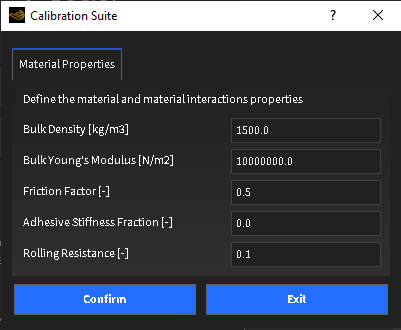
The pre-processing window essentially lists each deck’s input variables and separates them into three different tabs (when applicable): Material Properties, Operating Conditions and User Parameters.
If the user has no access to the GUI, e.g., when running in batch or headless modes, the input variables can also be modified by incluing a file named parametric_variables.json in the project’s folder.
If we consider some of the variables shown in Listing: parametric_variables.json, the file should look like the following:
 {
    ’rho’ : 1500,
    ’E’ : 1e7,
    ’ff’ : 0.5
 }
As seen in the file above, the user is not required to specify all the variables in the JSON file, only those the user is intended to change.
For running parametric studies, the user can leverage the new structure of the Calibration Suite and choose among the following:
Automate the modification of the parametric_variables.json file.
Modify the input variables directly with the aid of the API:PrePost.
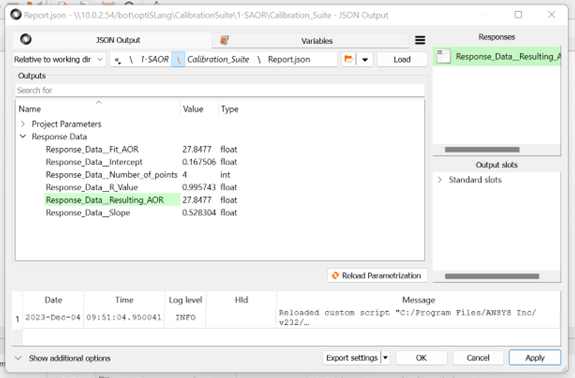
Use Ansys optiSLang integration. Please refer to section Figure 3.4: Reading the outputs from the Report.json file.
The Calibration Suite post-processing stage will execute specific post-processing routines for each Calibration Suite deck. Each deck has its own set of post-processing parameters, such as the number of divisions for an Eulerian Statistics user process, or the dimensions of its parent cube process. These parameters can only be modified, if necessary, through another JSON file located within the project’s folder, and named post_processing_parameters.json.
The details of this file corresponding to each Calibration Suite deck will be discussed in Calibration Suite Decks.
When the post-processing step is successfuly executed, a new folder named Calibration_Suite will be created within the project’s folder.
For each deck, at least three files will be always generated:
{deck_name}_raw_data.csv: Contains raw output data. This is intended to give the user the ability to perform its own data treatment.
Plot_{deck_name}.png: A graphical representation of the results (it can be a pile or stress consolidation plots).
Report.json: This is a JSON file carrying the input variable values, and also the relevant output quantities. Its purpose is to be easily readable by external scripts or Ansys optiSLang. In the case of one of the angle of repose experiments, it would look like in Listing: Report.json:
 {
    "Project Parameters": {
        "Bulk Density [kg/m3]": 1500.0,
        "Bulk Young’s Modulus [N/m2]": 10000000.0,
        "Friction Factor [-]": 0.5,
        "Adhesive Stiffness Fraction [-]": 0.0,
        "Rolling Resistance [-]": 0.1
    },
    "Response Data": {
        "Slope": 0.45974292585807974,
        "Intercept": 0.16264180094319539,
        "R-Value": 0.9993830705149718,
        "Number of points": 6,
        "Fit AOR": 24.69027217158696,
        "Resulting AOR": 24.69027217158696
    }
 }
Additional files can be generated during post-processing. The details can be found in Calibration Suite Decks.
All the Calibration Suite decks can be run directly within Ansys optiSLang to perform sensitivity analysis, optimization, create reduced-order models, etc.
Using the Wizard or the Solver Wizard, start a project using the Ansys Rocky solver, using the desired Calibration Suite deck, and follow the on-screen instructions (for more information, refer to Ansys optiSLang integration section in the Ansys Rocky installation guide.
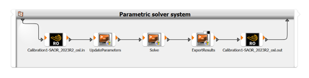
The default Parametric solver system template will collect output variables defined within Ansys Rocky. Since all the scripts generate a Report.json file, we can remove both the ExportResults and the (project-name).out modules and replace them with a JSON Output module. This module should receive designs from the Solve module and send them back to the parent system.
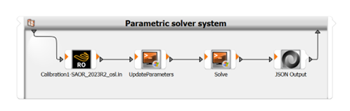
Edit the JSON Output module, selecting the report from the folder . . . \Calibration_Suite. Make sure that the path is set to Relativeto working dir and that the path split position is set before the Calibration_Suite folder. From the Outputs list, you can select any Response Data and use it as a Response for the project. After the selection of the responses, you can use the modified Parametric system to perform the desired analysis in Ansys optiSLang.