The Uncertainty Analysis will be performed through a series of runs corresponding to the set of collocation points generated based on the characteristics of the distributions of the uncertain input parameters. A separate subdirectory for each run will be created beneath the Project Working Directory. This Run Working Directory contains a copy of all needed input files and the output files generated by the run. The Solution Harvester is automatically invoked to collect solution data for user-specified output variables. A variance analysis is performed to study the contribution of each uncertain input parameter to the uncertainty of each user-selected output parameter. An error analysis is performed to determine the accuracy of the approximation model used in the uncertainty analysis. During post-processing of the Uncertainty Analysis, the Harvester is invoked to parse the solution files generated for each run and creates a merged solution set that can easily be analyzed using the visualization options of the Post-Processor.
Here, we use the project closed_homogeneous__transient.ckprj as an example of running an Uncertainty Analysis.
You can run the Uncertainty Analysis using the following steps:
Open the project closed_homogeneous__transient.ckprj and pre-process the chemistry set.
Follow the steps listed in Opening an Uncertainty Analysis Dialog for Reactor or Stream Properties and Setting up a Probability Distribution for an Uncertain Input Parameter to set up distributions for temperature and pressure.
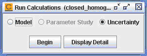
Double-click the Run Calculations node in the project tree. A Run Calculations panel will pop up in the interface, as shown in Figure 3.6: closed_homogeneous__transient.ckprj — Uncertainty Analysis.
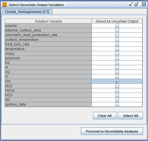
Click the Begin button. A Select Uncertain Output Variables panel will pop up in the interface, as shown in Figure 3.7: closed_homogeneous__transient.ckprj — Select Uncertain Output Variables Panel. You can use this panel to select the solution variables of interest. Click the Clear All button to deselect all variables and then select OH only. With this selection, we are going to study the effect of the variation in input values of reactor temperature and pressure on the final OH concentration in the reactor. If you are not sure which output variables are of most interest to you, you can just select all of them for now. You can always deselect uncertain output variables later on, as shown in the next steps. Click the Proceed to Uncertainty Analysis button.
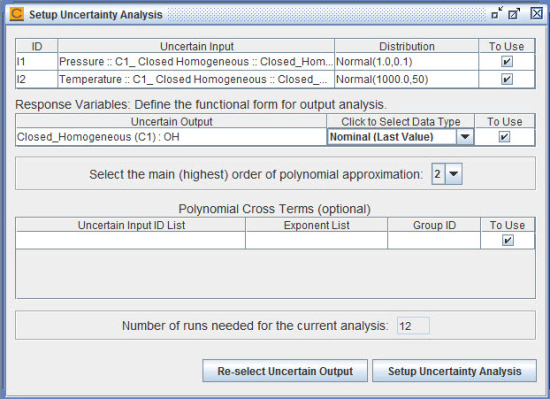
A Setup Uncertainty Analysis panel will pop up in the interface, as shown in Figure 3.8: closed_homogeneous__transient.ckprj — Setup Uncertainty Analysis Panel. This panel allows you to set up the Polynomial Chaos Expansions (PCE) of uncertain output variables.
As discussed in step 4, you can deselect any uncertain output (response) variables in this panel by unchecking the corresponding rows in the Response Variables table. You can also click the Re-select Uncertain Output button to re-run the nominal case and re-select the uncertain output variables. The second column of the Response Variables table is of particular importance here. As you know, this project is a transient calculation of a closed homogeneous batch reactor. A transient calculation will generate a vector of values for each output variable, one value per time point. However, the collocation calculation can use only a single value of each output variable. Therefore you must select which value or which type of combination of the values will be used in the calculation. You can click on an entry in the second column to select the type of data from a drop-down list. For OH concentration, we will use the default data type, that is, the nominal (last) value in the transient solution.
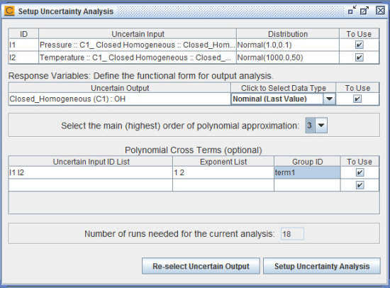
You can use the rest of the panel to set up the Polynomial Chaos Expansion (PCE) of uncertain output variable, OH concentration. You can select the highest order of polynomials used in the approximation of the uncertain output variable. Set the order to be 3. The Polynomial Cross Terms table is optional. If you think there is strong inter-dependency between the uncertain input parameters, you can use the polynomial cross terms to represent the dependency. In this case, we want a cross term that is first order on pressure and second order on temperature. Enter I1 I2 under the Uncertain Input ID List column and enter 1 2 under the Exponent List column. Provide an ID for this cross term by entering term1 under the Group ID column. The last sub-panel in the panel displays the total number of model runs that are required to complete the uncertainty analysis of OH concentration based on the current setup. Figure 3.9: closed_homogeneous__transient.ckprj — Final View of Setup Uncertainty Analysis Panel shows the final view of the panel. Click the Setup Uncertainty Analysis button to proceed.
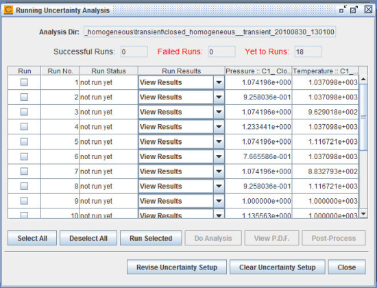
A Running Uncertainty Analysis panel will pop up in the interface, as shown in Figure 3.10: closed_homogeneous__transient.ckprj — Running Uncertainty Analysis Panel. This panel looks similar to the Run Parameter Study panel described in Section 3.3 of Chemkin Getting Started Guide. You can use this panel to launch jobs and process solutions.
Click the Select All button to select all runs. Click the Run Selected button to run all the jobs. It will create a new directory, closed_homogeneous__transient_########_######, in your Project Working Directory, with each directory date- and time-stamped. Each run creates a separate run directory named by the run number in this closed_homogeneous__transient_########_###### directory. During the runs, a Monitor Project Run panel will pop up in the interface, as shown in Figure 3.11: closed_homogeneous__transient.ckprj — Monitor Project Run Panel. This panel displays the current progress of the runs. If you want to stop early, you can click the Interrupt Jobs button to skip the runs that have not started yet. You can open this panel at any time by double-clicking on the Monitor Project Run node of the project tree. When all runs are done, close this panel by clicking the Close button.
When all the runs are complete, you will see the overall status displayed at the top of the Running Uncertainty Analysis panel as well as the Run Status column. To view the diagnostic output file and log file of each run, you can click the Click to View Results… pull-down list in the Run Results column.
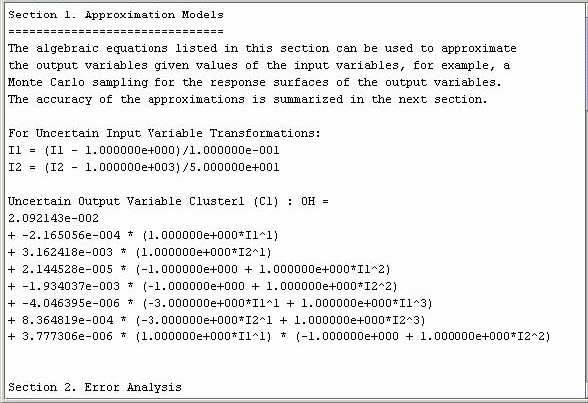
Click the Do Analysis button to perform the collocation calculation based on simulation results, the variance analysis, and the error analysis. A file editor will pop up in the interface displaying the results of the analysis, as shown in Figure 3.12: closed_homogeneous__transient.ckprj — Results of Variance Analysis and Error Analysis. The results contain three sections.
The first section displays the polynomial chaos expansion of the uncertain output variable, OH concentration in the reactor, in term of the uncertain input variables, reactor pressure and temperature.
The second section displays the results of the error analysis and lists suggestions on how to improve the accuracy.
The third section displays the results of the variance analysis and it shows that the variation in reactor pressure makes little contribution to the variation in OH concentration.
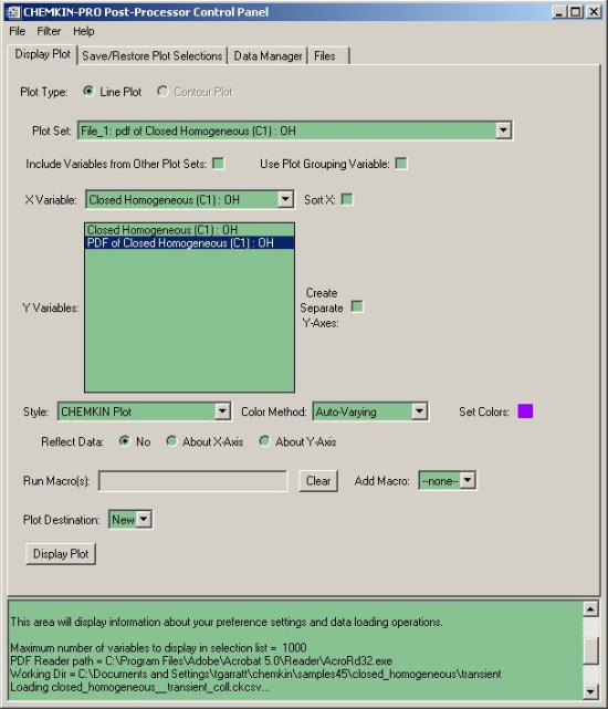
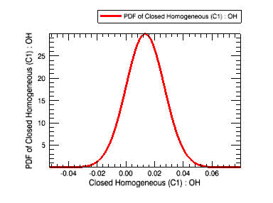
When the analysis is complete, the View P.D.F. button becomes active. Click the View P.D.F. button to view the plots of distributions of uncertain input and output variables. A Ansys Chemkin Post-Processor Control Panel will pop up as shown in Figure 3.13: closed_homogeneous__transient.ckprj — Post-Processor Control Panel. Click the Plot Set pull-down list to select pdf of Cluster1 (C1): OH. Click the Display Plot button to view the probability distribution of the OH concentration in the reactor at the last time point, as shown in Figure 3.14: closed_homogeneous__transient.ckprj — PDF of OH Concentration.
You can click the Post-Process button to process and display the results from all the runs. It is described in detail in Section 1.3 of Chemkin Getting Started Guide and the Chemkin Visualization Manual.
If you want to revise the setup of the uncertainty analysis, such as adjusting the order of the polynomial and adding/removing polynomial cross terms, you can click the Revise Uncertainty Setup button at the bottom of the Running Uncertainty Analysis panel to go back to the Setup Uncertainty Analysis panel displayed in Figure 3.9: closed_homogeneous__transient.ckprj — Final View of Setup Uncertainty Analysis Panel. Because of the nature of the collocation sampling points, different uncertainty setups usually share some sampling points. The Uncertainty Analysis Facility will automatically recycle the runs of these shared sampling points from a previous uncertainty setup, as long as they are saved in the project, so that you do not need to re-run these jobs.
If you want to remove all the distribution setups for uncertain input parameters and discard all the run results and analysis results of the uncertainty analysis, you can click the Clear Uncertainty Setup button at the bottom of the Running Uncertainty Analysis panel. This allows you to set up a new Uncertainty Analysis or a new Parameter Study from scratch.