


The Injection Distribution tab appears when, on the Injection Details tab,
Injection Model > Option is set to Cylindrical Hole.
The Injection Distribution setting controls whether a distribution function is applied to the variables near the injection positions.
The following topics are discussed:
For a cylindrical hole with a defined direction, you might want to control details about how mass is injected into the domain. In reality, the magnitude and direction of the fluid velocity might vary locally within the immediate vicinity of a hole exit, as would other quantities such as the local fluid temperature and turbulence intensity. These variations are a result of external conditions such as the relative velocity of any fluid already within the domain that is approaching the hole exit to form a cross-flow. These variations are also influenced by local geometry, such as the shape and direction of the hole. The settings on the Injection Distribution tab enable you to control details about how mass is injected into the domain and details about the local inflow conditions. As the mesh is refined near the injection positions, these local secondary flow patterns and condition variations can be resolved.
There is only one option for the type of injection distribution: Jet in Crossflow.
The Jet In Crossflow option assumes that the fluid from each hole is injected
from a boundary (that includes the hole exit) into a crossflow. However, the flow equation source terms
for mass, momentum, and so on, are applied throughout a small source volume near each hole exit.
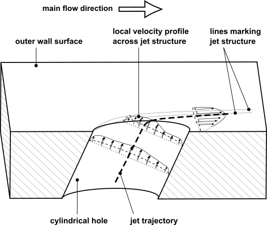
This source volume has a shape that approximates the jet structure. A typical jet structure bends with
the main flow direction after leaving a wall from an injection hole, and has varying velocity profiles
along its trajectory, as shown in Figure 18.1: Jet from a Wall into a Crossflow.
The Jet In Crossflow option has settings to specify:
A detail about the crossflow: the Inflow Boundary from which the crossflow originates
Details about how mass is injected: injection trajectory, injection shape, injection variables.
The exact shape of each hole source volume is described in terms of the injection trajectory and cross-sectional shape. Injection variables carry other properties of the jets.
The following topics are discussed:
The inflow boundary is the reference inlet for the domain. During a run, CFX-Solver uses this boundary to calculate the strength of the crossflow (local blowing ratio).
The injection trajectory is a curvilinear flow path that the fluid follows, the upstream end being within the hole and the downstream end being past the hole exit, out in the crossflow. The trajectory extends approximately one hole diameter upstream and downstream of the hole exit. Figure 18.1: Jet from a Wall into a Crossflow shows an example of an injection trajectory.
Injection Trajectory > Option
can only be set to Standard. This
trajectory model, which is described by auf dem Kampe, Völker,
and Zehe (2010) [231], takes into account:
The hole direction, which can be thought of as the direction of the drilling that created the hole (Injection Details tab > Injection Model > Hole Direction),
The crossflow conditions near the hole exit such as the local blowing ratio and the density ratio, and
The trajectory model parameters.
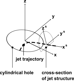
The trajectory is calculated in terms of local hole coordinates. These coordinates are shown in Figure 18.2: Local Hole Coordinates. The local x coordinate is parallel to the Hole Direction projected onto the boundary. The local z coordinate is normal to the boundary. The local y coordinate is transverse. The origin of the local hole coordinates is at the specified hole center position.
Note: Drilling paths that are precisely normal to the boundary should be avoided because they have an arbitrary local coordinate system. A small angle, for example 1 degree, should be used instead.

Inside the hole passage, the trajectory follows the drilling direction. In the region of the hole exit and beyond the hole exit, Equation 18–1 finds the y and z coordinates of points along the trajectory as a function of the local x coordinate.
 | (18–1) |
where:
 is the x-coordinate in local hole coordinates.
 stands for y when the equation is being solved for,
y-coordinates of the trajectory, or z when the equation is being solved
for z-coordinates of the trajectory.
stands for y when the equation is being solved for,
y-coordinates of the trajectory, or z when the equation is being solved
for z-coordinates of the trajectory. is Relative Offset Y
when the equation is being solved for
y-coordinates of the trajectory, or 0 (zero)
when the equation is being solved for
z-coordinates of the trajectory.
is Relative Offset Y
when the equation is being solved for
y-coordinates of the trajectory, or 0 (zero)
when the equation is being solved for
z-coordinates of the trajectory. is Relative Reference Y
when the equation is being solved for
y-coordinates of the trajectory, or Relative Reference Z
when the equation is being solved for
z-coordinates of the trajectory.
is Relative Reference Y
when the equation is being solved for
y-coordinates of the trajectory, or Relative Reference Z
when the equation is being solved for
z-coordinates of the trajectory. is A Coefficient Y
when the equation is being solved for
y-coordinates of the trajectory, or A Coefficient Z
when the equation is being solved for
z-coordinates of the trajectory.
is A Coefficient Y
when the equation is being solved for
y-coordinates of the trajectory, or A Coefficient Z
when the equation is being solved for
z-coordinates of the trajectory. is B Coefficient Y
when the equation is being solved for
y-coordinates of the trajectory, or B Coefficient Z
when the equation is being solved for
z-coordinates of the trajectory.
is B Coefficient Y
when the equation is being solved for
y-coordinates of the trajectory, or B Coefficient Z
when the equation is being solved for
z-coordinates of the trajectory. is the effective azimuthal angle
(Eff. Azimuthal Angle), which is
usually zero, when the equation is being solved for
y-coordinates of the trajectory, or the effective elevation angle (Eff.
Elevation Angle)
when the equation is being solved for
z-coordinates of the trajectory.
is the effective azimuthal angle
(Eff. Azimuthal Angle), which is
usually zero, when the equation is being solved for
y-coordinates of the trajectory, or the effective elevation angle (Eff.
Elevation Angle)
when the equation is being solved for
z-coordinates of the trajectory. is the local hole diameter.
 is the momentum ratio, which is automatically
derived from the local blowing ratio
and the local density ratio.
is the momentum ratio, which is automatically
derived from the local blowing ratio
and the local density ratio.
Relative Offset Y, Relative Reference Y, and Relative Reference Z dictate where the trajectory intersects the boundary at the hole exit. The A and B coefficients describe how the local y and local z coordinates change.
Under Spherical Angles, the effective angles describe the direction of the trajectory downstream of the hole exit:
The Effective Azimuthal Angle (Eff. Azimuthal Angle) measures the local direction of the jet trajectory, as an angle in the local xy plane, measured from the x-axis to the projection of the trajectory’s tangent line on the local xy plane .
The Effective Elevation Angle (Eff. Elevation Angle) measures the local direction of the jet trajectory, as an angle in the local xz plane, measured from the x-axis to the projection of the trajectory’s tangent line on the local xz plane.
You can optionally set a minimum value (Min. Elevation Angle) for the elevation angle. The trajectory is clipped if and where the effective elevation angle would become less than the set minimum, thereby preventing the trajectory from becoming parallel to the boundary. Too low an effective elevation angle could create numerical problems, especially if the trajectory were to lie flat on the boundary.
The jet structure, which forms the source volume, is constructed from a series of cross-sections that are perpendicular to the trajectory. The outline shape of these cross-sections are calculated according to the Injection Shape settings.
Figure 18.3: Local Hole Coordinates and a Jet Cross-section showing Cross-sectional Coordinates shows an example of a jet that has a simple circular cross-section. The cross section has its own coordinates, with xs being along the trajectory. Note that the cross-section shown in this example has a flat edge as a result of being truncated at the boundary. The Injection Shape settings control the shape of jet cross-section before any truncation by boundaries.
Injection Shape > Option
can only be set to Radial Fourier Series, where the
local cross-section radius around the trajectory is a function, in the
form of a truncated Fourier series, of the polar angle around the trajectory.
The cross-sections are mathematically modeled using
Equation 18–2:
 | (18–2) |
where:
 is Fourier A0 Coefficient,
 is Fourier A1 Coefficient,
 is Fourier B1 Coefficient,
 is Fourier A2 Coefficient,
 is Fourier B2 Coefficient,
 is the hole diameter,
 is the polar angle in the local yszs
plane, measured from the local ys-axis towards
the local zs-axis,
is the polar angle in the local yszs
plane, measured from the local ys-axis towards
the local zs-axis, is the cross-sectional radius in that direction,
 denotes the local trajectory frame.
The coefficients can be adjusted to fine tune the injection shape if required, and need not be constant.
Note that the coefficients of the Fourier series are normalized by the hole diameter. If, for example, the A0 coefficient is set to 1, and the other coefficients are set to 0, then the cross-sections are circular and centered on the trajectory, and the source volume for each hole is a truncated cylinder, possibly curved depending on the strength of the crossflow.
For each primitive solution variable relevant to the current simulation (for example, velocity, temperature, and so on) you can select an option to describe how that variable varies within the source volume at each hole.
There are several available options for specifying variations, as described in the following sections:
Each option either:
Defines a distribution function, where variations in scalars or vector magnitudes are expressed in terms of normalized values, or
Directly defines values for scalar quantities, vector magnitudes, or vector components.
For each injection variable controlled by a distribution function, the magnitude given by the distribution function is automatically scaled so that the net quantity applied over the source volume at each hole (for example momentum, enthalpy) is approximately constant irrespective of the form of the distribution function. Also, the velocity magnitude is scaled to be consistent with the mass flow. This scaling is done in a similar way to that shown by auf dem Kampe and Völker (2010) [232].
With the Uniform option, the variable has the same
value everywhere within the source volume.
Note that for a vector quantity such as velocity, the Uniform
option means that the magnitude is uniform; the direction
is always parallel to the trajectory.
The Quadratic Radial Polynomial option models variation of
a variable in the radial direction from the trajectory, using a quadratic function
operating on the normalized radial coordinate. In the case of a vector variable, this
distribution function dictates the magnitude of the vector. The direction is always
parallel to the tangent at the nearest point on the trajectory.
The equation for the model is shown in Equation 18–3.
 | (18–3) |
Here,  is the radial position from the trajectory
in the local trajectory frame, and
is the radial position from the trajectory
in the local trajectory frame, and  is the cross-sectional
radius in that frame (Equation 18–2). The ratio of the two therefore ranges from 0 to 1.
is the cross-sectional
radius in that frame (Equation 18–2). The ratio of the two therefore ranges from 0 to 1.
The model requires three dimensionless coefficients:
A Coefficientfor the constant,B Coefficientfor the first order term, andC Coefficientfor the second order term.
Note that setting these coefficients to 1,0,0, respectively, is effectively the same as choosing
the Uniform option (see Uniform).
You can specify the value(s) of a scalar variable using the Value option,
which allows a CEL expression. For example, you could use a CEL expression to specify a
position-dependent scalar value.
The Standard Jet Velocity option is available only for
vector variables (for example, Velocity) and is an
extension of the Quadratic Radial Polynomial option.
This option facilitates the setup of a counter-rotating vortex secondary flow pattern within the jet. The model for this flow pattern is described by auf dem Kampe, Völker, and Zehe (2010) [231].
The governing equations for the velocity components, us, vs, and ws, in cross-sectional coordinate directions xs, ys, and zs, respectively, are written as functions of transformed (in fact, rotated) ys and zs coordinates, called yr and zr, respectively, which are calculated as follows:
 | (18–4) |
Here,
 and
and  are angles used to rotate the local
 coordinate frame for the calculation of velocity components
  and
and
 respectively.
Using the transformed coordinates  and
and  ,
the velocity components are calculated using the following equations:
,
the velocity components are calculated using the following equations:
 | (18–5) |
where:
Coefficients
 ,
,  , and
, and  , are non-dimensional.
 ,
,  ,
,
 , and
, and  are parameters that affect the distributions of velocity components
  and
and  .
.
The Cartesian Vector Components option is available only
for vector variables.
Specify the vector components directly, optionally using CEL expressions.
The vector components, U, V, and
W, are aligned with the trajectory’s
x, y, and z axes, respectively.