


Near a no-slip wall, there are strong gradients in the dependent variables. In addition, viscous effects on the transport processes are large. The representation of these processes within a numerical simulation raises the following problems:
How to account for viscous effects at the wall.
How to resolve the rapid variation of flow variables that occurs within the boundary layer region.
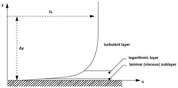
Experiments and mathematical analysis have shown that the near-wall region can be subdivided into two layers. In the innermost layer, the so-called viscous sublayer, the flow is almost laminar-like, and the (molecular) viscosity plays a dominant role in momentum and heat transfer. Further away from the wall, in the logarithmic layer, turbulence dominates the mixing process. Finally, there is a region between the viscous sublayer and the logarithmic layer called the buffer layer, where the effects of molecular viscosity and turbulence are of equal importance. The figure below illustrates these subdivisions of the near-wall region.
Assuming that the logarithmic profile reasonably approximates the velocity distribution near the wall, it provides a means to numerically compute the fluid shear stress as a function of the velocity at a given distance from the wall. This is known as a ‘wall function’ and the logarithmic nature gives rise to the well known ‘log law of the wall.’
Two approaches are commonly used to model the flow in the near-wall region:
The wall function method uses empirical formulas that impose suitable conditions near the wall without resolving the boundary layer, thus saving computational resources. All turbulence models in CFX are suitable for a wall function method.
The major advantages of the wall function approach is that the high gradient shear layers near walls can be modeled with relatively coarse meshes, yielding substantial savings in CPU time and storage. It also avoids the need to account for viscous effects in the turbulence model.
The Low-Reynolds-Number method resolves the details of the boundary layer profile by using very small mesh length scales in the direction normal to the wall (very thin inflation layers). Turbulence models based on the
 -equation, such as the SST or SMC-
 models,
are suitable for a low-Re method. Note that the low-Re method does not refer to the device Reynolds
number, but to the turbulent Reynolds number, which is low in the
viscous sublayer. This method can therefore be used even in simulations
with very high device Reynolds numbers, as long as the viscous sublayer
has been resolved.
models,
are suitable for a low-Re method. Note that the low-Re method does not refer to the device Reynolds
number, but to the turbulent Reynolds number, which is low in the
viscous sublayer. This method can therefore be used even in simulations
with very high device Reynolds numbers, as long as the viscous sublayer
has been resolved.The computations are extended through the viscosity-affected sublayer close to the wall. The low-Re approach requires a very fine mesh in the near-wall zone and correspondingly large number of nodes. Computer-storage and run-time requirements are higher than those of the wall-function approach and care must be taken to ensure good numerical resolution in the near-wall region to capture the rapid variation in variables. To reduce the resolution requirements, an automatic wall treatment was developed by CFX, which allows a gradual switch between wall functions and low-Reynolds number grids, without a loss in accuracy.
Wall functions are the most popular way to account for wall
effects. In CFX, Scalable Wall Functions are
used for all turbulence models based on the  -equation.
For
-equation.
For  based models (including the SST
model), an
based models (including the SST
model), an Automatic near-wall treatment method
is applied.