


There are predefined macros that are readily available in the
Macro Calculator. These predefined macros are provided in the form
of session files (file extension .cse) that are
located in
<CFDPOSTROOT>/etc/ and
that are loaded via
<CFDPOSTROOT>/etc/CFXPostInit.ccl upon starting CFD-Post.
Some macros produce an HTML-formatted report that can be viewed by clicking the View Report button or by opening the Report Viewer.
The following sections describe the predefined macros:
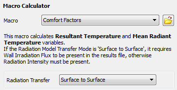
The Comfort Factors macro can be used to
calculate values for Resultant Temperature and Mean Radiant Temperature in HVAC simulations.
In order to use the macro, the velocity and temperature variables are required. In addition:
If Radiation Transfer is set to
Surface to Surfacethen variableWall Irradiation Fluxis required.If Radiation Transfer is set to
Participating Mediathen variableRadiation Intensityis required.
For CFX cases, the Radiation Transfer selection should match the radiation transfer mode used in the CFX-Solver. For non-CFX cases, the selection should depend on which radiation variables are available.
Variables Resultant Temperature and Mean Radiant Temperature are created using the values
of expressions resultTemp and meanTemp, respectively. These expressions are visible on the Expressions tab.
Note: As an alternative to calculating comfort factors in CFD-Post, the comfort factors may be calculated during the solution process; this would be required, for example, when the model simulates a ventilation system in which the control system depends dynamically on derived comfort factors.
Note: For more information regarding variables Wall
Irradiation Flux and Radiation Intensity, which may be used by the macro, see Variables Relevant for Radiation Calculations in the CFX Reference Guide.
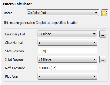
The Cp Polar macro produces a polar plot of the pressure coefficient (Cp) along a polyline. The macro creates the polyline using the Boundary Intersection method. For details, see Polyline Command. The boundary and intersecting slice plane are defined in the Macro Calculator and passed to the subroutine as arguments. The boundaries selected for Boundary List in the Macro Calculator make up one surface for the intersection. The second surface is a slice plane created using the X, Y, or Z normal axis to the plane (Slice Normal) and a point on that axis (Slice Position).
The cp user variable is created by the macro from the cp expression. The cp expression can be defined as:
(Pressure - $pref [Pa])/dynHead
where $pref is the Ref.
Pressure set in the Macro Calculator and dynHead is a reference dynamic head (evaluated at the inlet) that can be
defined as:
0.5 * areaAve(Density)@inlet * areaAve(Velocity)@inlet^2
The Inlet Region selected in the Macro
Calculator is used as the inlet location in the
calculation of dynHead.
Next, a Chart line of the cp variable versus the Plot X Axis value is created. The generated report contains the chart and the settings from the Macro Calculator.
The following information must be specified:
Boundary List: A list of boundaries used in the simulation.
Slice Normal: The axis that will be normal to the slice plane.
Slice Position: The offset of the slice plane in the direction specified by the normal axis.
Inlet Region: The locator used to calculate inlet quantities.
Ref. Pressure: The reference pressure for the simulation.
Plot Axis: The axis on which the results will be plotted.
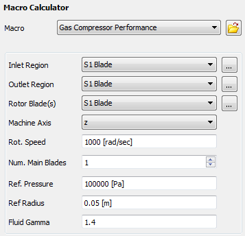
The Compressor Performance macro performs a series of calculations using the data set in the Macro Calculator. The following information must be specified:
Inlet Region: The locator used to calculate inlet quantities.
Outlet Region: The locator used to calculate outlet quantities.
Rotor Blade(s): The locator used to calculate torque (one blade row) about the machine axis.
Machine Axis: The axis of rotation of the compressor.
Rot. Speed: The rotational speed of the compressor.
Num. Main Blades: Some quantities calculated for a single blade set (main blade and any splitter blades) are multiplied by the number of blade sets in the full 360° wheel in order to produce the total value for the wheel.
Ref Pressure: The reference pressure for the simulation.
Ref Radius: A reference radius between the hub and tip.
Fluid Gamma: The ratio of specific heat capacity at constant pressure to specific heat capacity at constant volume (Cp / Cv).
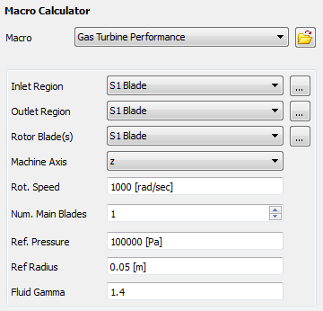
The following information must be specified:
Inlet Region: The locator used to calculate inlet quantities.
Outlet Region: The locator used to calculate outlet quantities.
Rotor Blade(s): The locator used to calculate torque (one blade row) about the machine axis.
Machine Axis: The axis or rotation of the turbine.
Rot. Speed: The rotational speed of the turbine.
Num. Main Blades: Some quantities calculated for a single blade set (main blade and any splitter blades) are multiplied by the number of blade sets in the full 360° wheel in order to produce the total value for the wheel.
Ref Pressure: The reference pressure for the simulation.
Ref Radius: Reference radius between the hub and tip.
Fluid Gamma: The ratio of specific heat capacity at constant pressure to specific heat capacity at constant volume (Cp / Cv).
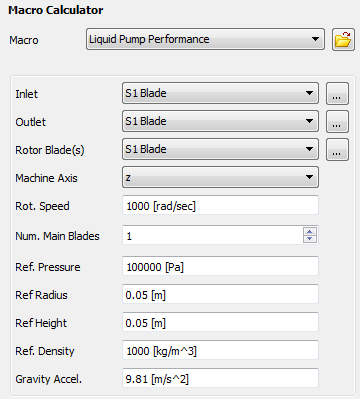
The following information must be specified:
Inlet: The locator used to calculate inlet quantities.
Outlet: The locator used to calculate outlet quantities.
Rotor Blade(s): The locator(s) used to calculate torque (one blade row) about the machine axis.
Machine Axis: The axis or rotation of the pump.
Rot. Speed: The rotational speed of the pump.
Num. Main Blades: Some quantities calculated for a single blade set (main blade and any splitter blades) are multiplied by the number of blade sets in the full 360° wheel in order to produce the total value for the wheel.
Ref Pressure: The reference pressure for the simulation.
Ref Radius: Reference radius between the hub and tip.
Ref Height: Cross-section height (that is, the height of the outlet region, or the height of the blade at the trailing edge).
Ref Density: The reference density for the simulation.
Gravity Accel.: The acceleration due to gravity.
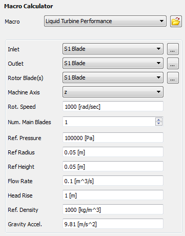
The following information must be specified:
Inlet: the locator used to calculate inlet quantities.
Outlet: the locator used to calculate outlet quantities.
Rotor Blade(s): the locators used to calculate torque (one blade row) about the machine axis.
Machine Axis: the axis or rotation of the turbine.
Rot. Speed: the rotational speed of the turbine.
Num. Main Blades: Some quantities calculated for a single blade set (main blade and any splitter blades) are multiplied by the number of blade sets in the full 360° wheel in order to produce the total value for the wheel.
Ref Pressure: The reference pressure for the simulation.
Ref Radius: reference radius between the hub and tip.
Ref Height: Cross-section height (that is, the height of the outlet region, or the height of the blade at the trailing edge).
Flow Rate: The volume flow rate.
Head Rise: The pressure head at the inlet.
Ref Density: The reference density for the simulation.
Gravity Accel.: The acceleration due to gravity.
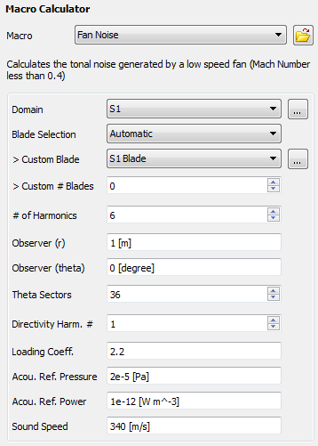
This macro calculates the noise levels of the turbomachinery as observed at a specific location. The following information must be specified:
Domain: The domain in which the blade is located.
Blade Selection: Set to Automatic for a single blade passage or Custom for a multiple blade passage. If this is set to
Custom, you will need to specify the 2D region for the blade (Custom Blade) as well as the number of blades (Custom # Blades).# of Harmonics: The number of harmonics used in the calculation.
Observer (r) and Observer (theta): The distance and location of the observer, relative to the blade.
Theta Sectors: The number of sampling points (sectors) equally spaced over 360° at a given radius around the fan, used to calculate the noise values. A higher number leads to a more accurate solution, but takes more time to calculate.
Directivity Harm. #: The harmonic level at which the sound pressure levels will be calculated.
Loading Coeff.: A coefficient between 2 and 2.5.
The loading coefficient parameter defines the decay (or decrease) of the sound-pressure level vs the frequency. In general, the sound-pressure level decreases when the frequency increases. In his experiments, Lowson replaced the unsteady loading by a steady one multiplied by a decay function. Based on these experiments, this decay follows an exponential law with a negative slope. Lowson found that a loading coefficient between 2 and 2.5 gives a sound-pressure level close to the experimental data; that is, the loading coefficient defines the slope of the exponential law.
In general and for highly loaded blades, the decay of the sound-pressure level is very quick (one or two peaks in the sound-pressure level spectrum) and therefore a higher value of the loading coefficient will be appropriate.
Acou. Ref. Pressure: Acoustic reference pressure (
 ) is the international standard for the minimum audible
sound of 2.10-5 [Pa].
) is the international standard for the minimum audible
sound of 2.10-5 [Pa]. The acoustic reference pressure is used to convert the acoustic pressure into Sound Pressure in dB using the following equation:

(13–1)
where
 is the acoustic
reference pressure. The reference pressure depends on the fluid.
is the acoustic
reference pressure. The reference pressure depends on the fluid.Acou. Ref. Power: Acoustic reference power (
 ) is used to convert the sound power
  from units of
  to units of dB.
The equation used is:

(13–2)
where:
The acoustic reference power is:

Sound Speed: The speed of the sound in the fluid at rest.


For details on completing this dialog box, see Using the Fan Noise Macro.
The Fan Noise macro calculates the tonal noise levels generated by a low-speed fan (primarily axial-flow fans). Tonal noise, or discrete-frequency noise, is due mainly to periodic forces exerted on fluid passing a fan. The Fan Noise macro can be applied to low speed fans having a tip Mach number less than 0.45. For a higher tip Mach number, the accuracy of the results is questionable. The fan must radiate in the free field where the observer can see the fan blades (the Fan Noise macro does not take into account the reflection effect). Thus, the Fan Noise macro cannot be applied to ducted fans.
The following topics are discussed:
Several methods have been developed to predict tonal noise; the Lowson Model is described here.
In the low-speed regime, the main noise component is a dipolar
source. Lowson [Lowson, M. V., 1970, "Theoretical
analysis of compressor noise", The Journal of Acoustics
So. Am., Vol. 47 (1), 1970, pp. 371-385.] showed that the noise generated
by a fan is directly related to the aerodynamic forces exerted on
the fixed and rotating blades. First, in a semi-empirical way, he
calculated these forces; then he took into account the distance between
the source and the observer. In this case, the fan is considered as
a noise source for which the frequency depends on the rotational speed
and other parameters. In 1962, Lighthill established the acoustic
pressure expression produced by a punctual force,  , in rectilinear motion.
 | (13–4) |
where:


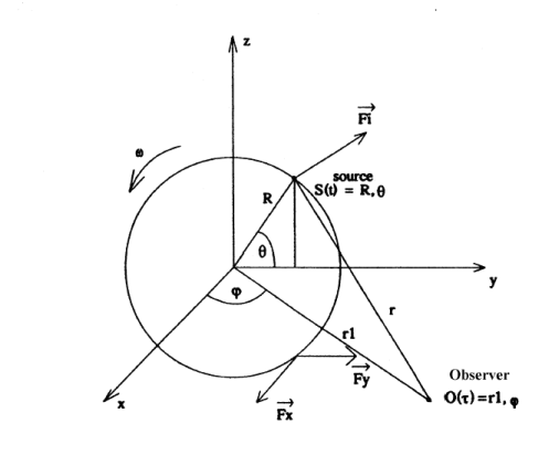
As shown in Figure 13.1: Relative position of the source and the observer,  and
and  are the coordinates of the Observer O (r,
  ,
,  ) and
of the Source S (R,
) and
of the Source S (R,  , t), respectively.
  is the convective component of the rotational Mach
number in the
is the convective component of the rotational Mach
number in the  direction.
  and
and  are respectively the thrust and the drag (torque)
forces exerted on the blade. According to Equation 13–4, when the force
are respectively the thrust and the drag (torque)
forces exerted on the blade. According to Equation 13–4, when the force  is
constant, the acoustic pressure is equal to zero.
is
constant, the acoustic pressure is equal to zero.
Lowson extended Equation 13–4 to create a more general equation:
 | (13–5) |
This relation describes the contribution of the convective phenomenon
due to the term  . Note that Equation 13–5 must be evaluated at retarded time
  . This
equation can be used to find an expression for the sound from a point
force in arbitrary harmonic motion.
. This
equation can be used to find an expression for the sound from a point
force in arbitrary harmonic motion.
The Lowson model enables the calculation, at the observer position, of the acoustic pressure generated by steady and unsteady efforts. The latter are considered as punctual sources and correspond to the loads exerting by the z blades of the rotor. Lowson integrated Equation 13–5 in time and space to get the mth harmonic of the acoustic pressure generated by a periodic rotating loading:
 | (13–6) |
using the following equation:
 | (13–7) |
and integrating Equation 13–6 by parts gives:
 | (13–8) |
as shown in Figure 13.1: Relative position of the source and the observer with  being the axis of rotation and the fluctuating loading
and observer position being defined as:
being the axis of rotation and the fluctuating loading
and observer position being defined as:


In
 | (13–9) |
 and
and  are respectively the thrust and drag (torque) components
of the aerodynamic unsteady force represented by a global force exerted
on the blade.
are respectively the thrust and drag (torque) components
of the aerodynamic unsteady force represented by a global force exerted
on the blade.The terms in
 and
and  are important only in the acoustic near field. Thus,
in the acoustic far field, Equation 13–8 becomes:
are important only in the acoustic near field. Thus,
in the acoustic far field, Equation 13–8 becomes:
(13–10)
Taking into account of the thrust and drag periodicities, Lowson proposed the following formulation:
 | (13–11) |
where  is the effort harmonic order or
the mode.
is the effort harmonic order or
the mode.
Substituting the results obtained from Equation 13–9 and Equation 13–11 into Equation 13–10 gives:
 | (13–12) |
where the rotational Mach number is 
The integrals in Equation 13–12 can be identified as Bessel functions, and, using the expressions:
 | (13–13) |
Equation 13–12 can be evaluated directly to give the sound level radiated from z rotor blades:
 | (13–14) |
where:
 is a first Bessel Function of order
 is the number of blades
The interest of this relation is the knowledge of the components
of the fluctuating efforts  and
and  .
.
Following the experimental work done on helicopter blades by Scheiman [Scheiman, J., 1964, "Sources of noise in axial flow fans", Journal of Sound and Vibration, Vol. 1, (3), 1964, pp. 302-322.], Lowson extended Equation 13–14 to an equation that relates the steady-state components of the force to the acoustic pressure.
The Fan Noise macro calculates the tonal noise levels generated by a fan as heard at a specific location. To access the Fan Noise macro:
Load the
.resfile into CFD-Post.Click the Calculators tab.
In the Macro field, select
Fan Noise.In the Macro Calculator, specify the information described in Fan Noise Macro.
When the Macro Calculator fields are filled in, click .
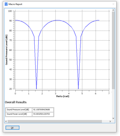
The Fan Noise macro outputs a report; to view it, click . The report displays the input values, the sound pressure levels, the sound power levels, the directivity of harmonic 1, and the overall results. Here is a partial sample:
The turbo noise report will be created in your working directory
as turboNoise_report.html along with the
tables (turboNoise_*.csv) and graphics (turboNoise_*.png) included in the report. This enables
you to reuse these elements in other documents, if required.
There are two ways to perform turbo noise calculations; you can have:
A case with a single blade passage (the Lowson model is based on this)
A case with a multiple blade passage, including a 360° case.
As shown below, the only necessary differences in the two cases are the settings for Blade Selection and the custom blade fields.
| Fan Noise Macro Values | Single Blade Passage | Multiple Blade Passage |
|---|---|---|
| Domain | Fan Block | Fan Block |
| Blade Selection | Automatic | Custom |
| > Custom Blade | Blade | |
| > Custom # of Blades | 9 | |
| # of Harmonics | 6 | 6 |
| Observer (r) | 1 m | 1 m |
| Observer (theta) | 0 degree | 0 degree |
| Theta Sectors | 36 | 36 |
| Directivity Harm. # | 1 | 1 |
| Loading Coeff. | 2.2 | 2.2 |
| Acou. Ref. Pressure | 2e-005 Pa | 2e-005 Pa |
| Acou. Ref. Power | 1e-012 W m^-3 | 1e-012 W m^-3 |
| Sound Speed | 340 m/s | 340 m/s |
To view the report, click Calculate and then View Report.