


VM-NR6645-01-1-a
VM-NR6645-01-1
VM-NR6645-01-1-a
Overview
Test Case
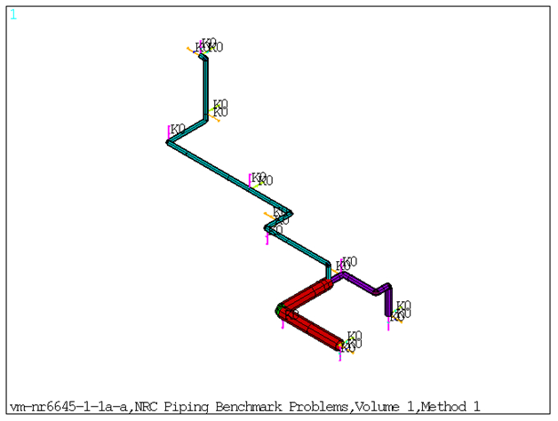
The schematic of the BM3 piping model is shown in Figure 619: FE Model of Benchmark Problem. The piping model is supported by means of elastic spring-damped elements. Modal and spectrum analysis is performed on the piping model. Lumped mass matrix formulation is used in the analysis. The first 14 modes obtained from modal solve is used in the subsequent spectrum analysis which is performed with an acceleration input spectra defined by 75 points. The model is excited in global X direction and the modes are combined using SRSS combination method. The spectrum solution is performed for two cases.
Spectrum solutions are performed for two cases:
Case 1: With missing mass effect (ZPA = 0.54g)
Case 2: With missing mass effect (ZPA = 0.54g) and rigid responses effect (Lindley method) Frequencies obtained from modal solve and reaction forces obtained from spectrum solve are compared against reference results.
| Material Properties | Geometric Properties | Loading | ||||||||||||||||||||||||||||||
|---|---|---|---|---|---|---|---|---|---|---|---|---|---|---|---|---|---|---|---|---|---|---|---|---|---|---|---|---|---|---|---|---|
Pipe Elements:
Density for different material ID: Material ID 1:
Material ID 2:
Material ID 3:
Material ID 4:
Material ID 5:
Material ID 6:
Stiffness for Spring-Damper Element: (lb/in) Since there are multiple Spring Supports at different locations, the Stiffness for the Spring Damper Elements are listed based on real constant set number. Set 7:
Set 8:
Set 9:
Set 10:
Set 11:
Set 12:
| Straight Pipe: Set 1:
Set 2:
Set 3:
Bend Pipe Elements: Set 4:
Set 5:
Set 6:
| Acceleration response spectrum curve defined by SV and FREQ commands. |
Results Comparison
Table 92: Frequencies Obtained from Modal Solution
| Mode | Target | Mechanical APDL | Ratio |
|---|---|---|---|
| 1 | 2.910 | 2.906 | 0.999 |
| 2 | 4.390 | 4.383 | 0.999 |
| 3 | 5.520 | 5.515 | 0.999 |
| 4 | 5.700 | 5.701 | 1.000 |
| 5 | 6.980 | 6.978 | 1.000 |
| 6 | 7.340 | 7.342 | 1.000 |
| 7 | 7.880 | 7.877 | 1.000 |
| 8 | 10.300 | 10.396 | 1.009 |
| 9 | 11.060 | 11.062 | 1.000 |
| 10 | 11.230 | 11.232 | 1.000 |
| 11 | 11.500 | 11.532 | 1.003 |
| 12 | 12.430 | 12.455 | 1.002 |
| 13 | 13.880 | 13.964 | 1.006 |
| 14 | 16.120 | 16.092 | 0.998 |
Reaction Forces Obtained from Spectrum Solve
Table 93: Case 1: With Missing Mass Effect (ZPA = 0.54g)
| Force_Node | Target | Mechanical APDL | Ratio |
|---|---|---|---|
| Fx at node1 | 48.081 | 48.1800 | 1.002 |
| Fy at node1 | 5.494 | 5.1448 | 0.937 |
| Fz at node1 | 7.584 | 6.9158 | 0.912 |
| Fx at node4 | 93.432 | 92.1492 | 0.986 |
| Fz at node4 | 75.438 | 68.8216 | 0.912 |
| Fy at node7 | 15.924 | 16.0453 | 1.008 |
| Fy at node11 | 19.699 | 19.8697 | 1.009 |
| Fz at node11 | 80.527 | 78.5385 | 0.975 |
| Fx at node15 | 438.882 | 435.6856 | 0.993 |
| Fy at node17 | 48.896 | 48.9000 | 1.000 |
| Fz at node17 | 79.739 | 79.0666 | 0.992 |
| Fy at node36 | 90.112 | 94.9487 | 1.054 |
| Fz at node36 | 85.082 | 87.6852 | 1.031 |
| Fx at node38 | 651.640 | 621.1533 | 0.953 |
| Fy at node38 | 52.562 | 53.3979 | 1.016 |
| Fz at node38 | 41.930 | 40.0603 | 0.955 |
| Fx at node23 | 264.782 | 260.2601 | 0.983 |
| Fy at node23 | 105.363 | 112.0384 | 1.063 |
| Fx at node31 | 50.646 | 50.1255 | 0.990 |
| Fy at node31 | 24.798 | 24.6392 | 0.994 |
| Fz at node31 | 31.678 | 30.9950 | 0.978 |
Table 94: Case 2: With Missing Mass Effect (ZPA = 0.54g) and Rigid Responses Effect (Lindley Method)
| Result | Target | Mechanical APDL | Ratio |
|---|---|---|---|
| Fx at node1 | 46.333 | 46.216 | 0.997 |
| Fy at node1 | 3.706 | 3.5776 | 0.965 |
| Fz at node1 | 3.536 | 3.2326 | 0.914 |
| Fx at node4 | 93.432 | 104.6064 | 0.995 |
| Fz at node4 | 36.218 | 33.2502 | 0.918 |
| Fy at node7 | 13.934 | 13.9509 | 1.001 |
| Fy at node11 | 15.173 | 15.2120 | 1.003 |
| Fz at node11 | 70.766 | 70.1082 | 0.991 |
| Fx at node15 | 592.491 | 586.3127 | 0.990 |
| Fy at node17 | 36.352 | 36.3426 | 1.000 |
| Fz at node17 | 63.399 | 62.8875 | 0.992 |
| Fy at node36 | 63.032 | 66.0934 | 1.049 |
| Fz at node36 | 53.914 | 54.4573 | 1.010 |
| Fx at node38 | 768.789 | 746.3653 | 0.971 |
| Fy at node38 | 47.784 | 48.0981 | 1.007 |
| Fz at node38 | 38.037 | 36.5269 | 0.960 |
| Fx at node23 | 342.659 | 338.8705 | 0.989 |
| Fy at node23 | 55.811 | 60.6286 | 1.086 |
| Fx at node31 | 56.151 | 56.6833 | 1.009 |
| Fy at node31 | 17.854 | 17.8872 | 1.002 |
| Fz at node31 | 22.994 | 22.4445 | 0.976 |