VM186
VM186
Transient Analysis of a Slot Embedded Conductor
Overview
Test Case
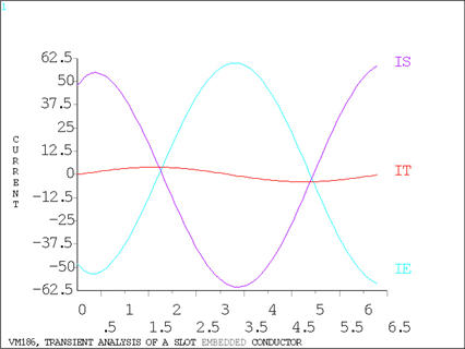
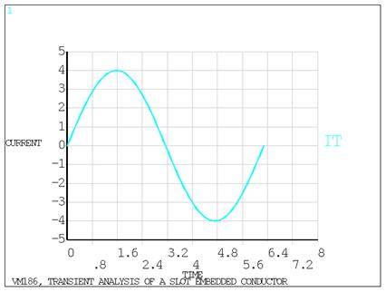
A solid conductor embedded in the slot of a steel electric machine carries a sinusoidally varying current I. Determine the vector magnetic potential solution after 3/4 and 1 period of the oscillation frequency. In addition, display the time-varying behavior of the total input current, the source current component, and the eddy current component.

| Material Properties | Geometric Properties | Loading | ||||||||
|---|---|---|---|---|---|---|---|---|---|---|
|
|
|
Analysis Assumptions and Modeling Notes
The slot is assumed to be infinitely long so that end effects are ignored, allowing for a two-dimensional planar analysis. An assumption is made that the steel containing the slot is infinitely permeable and so is replaced with a flux-normal boundary condition. It is also assumed that the flux is contained within the slot, so a flux-parallel boundary condition is placed along the top of the slot. The problem is stated in non-dimensional terms with properties given as unit values to match the reference.
The problem requires a coupled electromagnetic field analysis using the VOLT and AZ degrees of freedom. All VOLT DOF's within the conductor are coupled together to enforce the correct solution of the source current density component of the total current density. The eddy current component of the total current density is determined from the AZ DOF solution. The current is applied to a single arbitrary node in the conductor, since they are all coupled together in VOLT.
An initial solution is performed at a very small time step of 1 x 10⁻⁸ sec to establish a null field solution. Since no nonlinear properties are present, the NEQIT command is set to 1.0, suppressing equilibrium iterations at each time point. Eighty-one load steps are set up at constant time increments to accurately model the time-varying field solution. The Jacobian solver option is arbitrarily chosen.
PLANE13 elements can be used to output the eddy (IE), source (IS), and total current (IT), but PLANE233 can only output the total current (IT).
Results Comparison
| Vector Potential | Target | Mechanical APDL | Ratio |
|---|---|---|---|
| PLANE13 | |||
| @ node 1 (t = 3pi/2) | -15.18 | -15.07 | 0.993 |
| @ node 4 (t = 3pi/2) | -14.68 | -14.65 | 0.998 |
| @ node 7 (t = 3pi/2) | -4.00 | -4.00 | 1.00 |
| @ node 1 (t = 2pi) | -3.26 | -3.10 | 0.950 |
| @ node 4 (t = 2pi) | -0.92 | -0.89 | 0.966 |
| @ node 7 (t = 2pi) | 0 | 0 | 1.000 |
| PLANE233 | |||
| @ node 1 (t = 3pi/2) | -15.18 | -15.07 | 0.993 |
| @ node 4 (t = 3pi/2) | -14.68 | -14.65 | 0.998 |
| @ node 7 (t = 3pi/2) | -4.00 | -4.00 | 1.00 |
| @ node 1 (t = 2pi) | -3.26 | -3.10 | 0.950 |
| @ node 4 (t = 2pi) | -0.92 | -0.89 | 0.966 |
| @ node 7 (t = 2pi) | 0 | 0 | 1.000 |