VM167

VM167
Transient Eddy Currents in a Semi-Infinite Solid

Overview

Reference:

J. P. Holman, Heat Transfer, 4th Edition, McGraw-Hill Book Co., Inc., New York, NY, 1976, pg. 104, eqn. 4-14 (analogous field solution).

Analysis Type(s):

Transient Magnetic Field Analysis (ANTYPE = 4)

Element Type(s):

2D Coupled-Field Solid Elements (PLANE13)

2D 8-Node Electromagnetic Solid (PLANE233)

Input Listing:

vm167.dat

Test Case

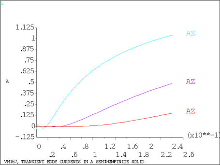
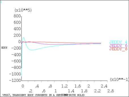
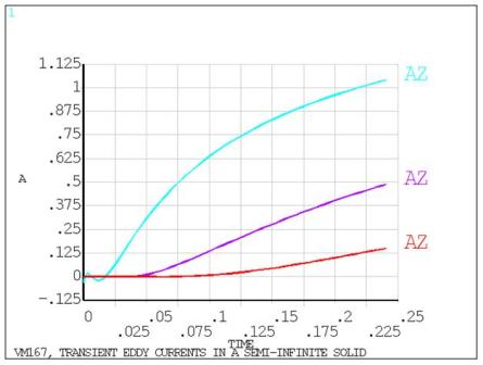
A semi-infinite solid is initially under no external magnetic field (vector potential A is zero throughout). The surface is suddenly subjected to a constant magnetic potential A_o. Determine the eddy current density, flux density and the vector potential field solution in the solid during the transient.

Figure 236: Semi-Infinite Solid Transient Eddy Currents Problem Sketch

Material Properties

Geometric Properties

μ = 4 π x 10^-7 H/m

ρ = 4 x 10^-7 ohm-m

= 20 m

h = 0.4 m

A_o = 2.0 Wb/m

Analysis Assumptions and Modeling Notes

A 0.4m² area is arbitrarily selected for the elements. The model length (20 m) is arbitrarily selected such that no significant potential change occurs at the end points (nodes 41, 91) for the time period of interest. The node locations are defined with a higher density near the surface to accurately model the transient behavior.

The transient analysis makes use of automatic time step optimization over a time period of 0.24 sec. A maximum time step size ((.24/48) = .005 sec.) is based on δ²/4 α, where δ is the conduction length within the first element (δ = .0775m) and α is the magnetic diffusivity (α = ρ / μ = .31822 m²/sec.). The minimum time step (.0002 sec) is selected as 1/25 of the maximum time step. The starting time step of 0.0002 sec. is arbitrarily selected. The problem is solved with two load steps to provide solution output at the desired time points. In the first load step, the step potential load is applied while setting initial boundary conditions of zero at all other potentials. The problem is first solved with PLANE13 elements and then using PLANE233 elements. The eddy current density output is not available with PLANE233.

Results Comparison

t = 0.15 sec	Target	Mechanical APDL	Ratio
PLANE13
Vector Potential (Wb/m)
@ x = 0.2517	0.831	0.822	0.990
@ x = 0.4574	0.282	0.275	0.975
@ x = 0.6914	0.050	0.0474	0.9337
Flux Density (T)
@ x = 0.2517	3.707	3.680	0.993
@ x = 0.4574	1.749	1.760	1.006
@ x = 0.6914	0.422	0.449	1.065
Eddy Current Density (x 10⁷ A/m²)
@ x = 0.2517	-0.777	-0.795	1.023
@ x = 0.4574	-0.663	-0.66	1.006
@ x = 0.6914	-0.243	-0.238	0.979
PLANE233
Vector Potential (Wb/m)
@ x = 0.2517	0.831	0.822	0.990
@ x = 0.4574	0.282	0.275	0.975
@ x = 0.6914	0.050	0.0474	0.937
Flux Density (T)
@ x = 0.2517	3.707	3.680	0.993
@ x = 0.4574	1.749	1.760	1.006
@ x = 0.6914	0.422	0.449	1.065

Figure 237: Vector Potential vs. Time Plot using PLANE13 Elements

Figure 238: Eddy Current Density vs. Time Plot using PLANE13 Elements

Figure 239: Vector Potential vs. Time Plot using PLANE233 Elements