In this sample problem, you will analyze the buckling of a bar with hinged ends.
Determine the critical buckling load of an axially loaded long slender bar of
length  with hinged ends. The bar has a cross-sectional height h, and area
A. Only the upper half of the bar is modeled because of symmetry. The boundary
conditions become free-fixed for the half-symmetry model. The moment of inertia of
the bar is calculated as I = Ah2/12 = 0.0052083
in4.
with hinged ends. The bar has a cross-sectional height h, and area
A. Only the upper half of the bar is modeled because of symmetry. The boundary
conditions become free-fixed for the half-symmetry model. The moment of inertia of
the bar is calculated as I = Ah2/12 = 0.0052083
in4.
The model is assumed to act only in the X-Y plane.
The following material properties are used:
| E = 30 x 106 psi |
The following geometric properties are used:
 = 200 in = 200 in |
| A = 0.25 in2 |
| h = 0.5 in |
Loading is a follows:
| F = 1 lb. |

After you enter the Mechanical APDL program, follow these steps to set the title.
Select menu path .
Enter the text "Buckling of a Bar with Hinged Ends" and click on OK.
In this step, you define BEAM188 as the element type.
Select menu path . The Element Types dialog box appears.
Click Add. The Library of Element Types dialog box appears.
In the scroll box on the left, click on "Structural Beam" to select it.
In the scroll box on the right, click on "2 Node 188" to select it.
Click OK. The Library of Element Types dialog box closes.
Click Options in the Element Types dialog box.
Select Element Behavior K3 : Cubic Form. Click OK.
Click Close in the Element Types dialog box.
Select menu path . The BeamTool dialog box appears.
Enter .5 for B and .5 for H.
Click OK.
Select menu path . The Define Material Model Behavior dialog box appears.
In the Material Models Available window, double-click on the following options: Structural, Linear, Elastic, Isotropic. A dialog box appears.
Enter 30e6 for EX (Young's modulus), and click on OK. Material Model Number 1 appears in the Material Models Defined window on the left.
Select menu path to remove the Define Material Model Behavior dialog box.
Select menu path . The Create Nodes in Active Coordinate System dialog box appears.
Enter 1 for node number.
Click Apply. Node location defaults to 0,0,0.
Enter 11 for node number.
Enter 0,100,0 for the X, Y, Z coordinates.
Click OK. The two nodes appear in the Graphics window.
Note: The triad, by default, hides the node number for node 1. To turn the triad off, select menu path and select the "Not Shown" option for Location of triad. Then click OK to close the dialog box.
Select menu path . The Fill between Nds picking menu appears.
Click on node 1, then 11, and click on OK. The Create Nodes Between 2 Nodes dialog box appears.
Click OK to accept the settings (fill between nodes 1 and 11, and number of nodes to fill 9).
Select menu path . The Elements from Nodes picking menu appears.
Click on nodes 1 and 2, then click on OK.
Select menu path . The Copy Elems Auto-Num picking menu appears.
Click Pick All. The Copy Elements (Automatically-Numbered) dialog box appears.
Enter 10 for total number of copies and enter 1 for node number increment.
Click OK. The remaining elements appear in the Graphics window.
Select menu path . The New Analysis dialog box appears.
Click OK to accept the default of "Static."
Select menu path . The Static or Steady-State Analysis dialog box appears.
To include prestress effects, click the check box to "YES" for "[PSTRES] Incl prestess effects?"
Click OK.
Select menu path . The Apply U,ROT on Nodes picking menu appears.
Click on node 1 in the Graphics window, then click on OK in the picking menu. The Apply U,ROT on Nodes dialog box appears.
Click on "UY" and “ROTZ” to select them, and click on OK.
Select menu path . The Apply U,ROT on Nodes picking menu appears.
Click on node 11 in the Graphics window, then click on OK in the picking menu. The Apply U,ROT on Nodes dialog box appears.
Click on "UX" to select it, and click on OK.
Select menu path . The Apply F/M on Nodes picking menu appears.
Click on node 11, then click OK. The Apply F/M on Nodes dialog box appears.
In the scroll box for Direction of force/mom, scroll to "FY" to select it.
Enter -1 for the force/moment value, and click on OK. The force symbol appears in the Graphics window.
Select menu path . The Apply SYMM on Nodes box dialog appears.
In the scroll box for Norml symm surface is normal to, scroll to “z-axis” and click on OK.
Select menu path .
Carefully review the information in the status window, and click on Close.
Click OK in the Solve Current Load Step dialog box to begin the solution.
Click Close in the Information window when the solution is finished.
Select menu path .
In the New Analysis dialog box, click the "Eigen Buckling" option on, then click on OK.
Note: Click Close in the Warning window if the following warning appears: Changing the analysis type is only valid within the first load step. Pressing OK will cause you to exit and reenter SOLUTION. This will reset the load step count to 1.
Select menu path . The Eigenvalue Buckling Options dialog box appears.
Enter 1 for number of modes to extract.
Click OK.
Select menu path .
Enter 1 for number of modes to expand, and click on OK.
Select menu path .
Carefully review the information in the status window, and click on Close.
Click OK in the Solve Current Load Step dialog box to begin the solution.
Click Close in the Information window when the solution is finished.
Select menu path .
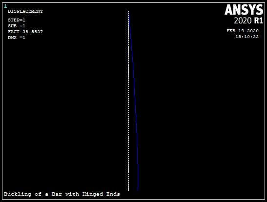
Select menu path . The Plot Deformed Shape dialog box appears.
Click the "Def + undeformed" option on. Click OK. The deformed and undeformed shapes appear in the Graphics window as seen in Figure 7.4: Buckling Analysis: Deformed and Undeformed Shapes.