


In this section we describe in detail the implementation of a quadratic limit surface used to model the anisotropic hardening behavior observed in some composite materials.
There are perhaps two definitions for failure; for a structural designer failure may be considered the point at which the material starts to become nonlinear (due to plasticity or micro-cracking, for example), however for the simulation of extreme loading events such as HVI failure is considered to be the point at which the material actually ruptures (becomes perforated). To get to this point, the material transitions elastic to inelastic deformation (due to micro-cracking, plasticity in the matrix or re-orientation of fibers) and finally reaches ultimate failure. We take the later definition, and for the purposes of this model we will term this nonlinear stress strain behavior “hardening” (see Figure 3.1: Typical In-Plane Stress-Strain Behavior of Kevlar-Epoxy).
The anisotropic yield criteria of Tsai-Hill can be used to represent the potentially different limits in elastic material behavior in the three orthotropic material directions [5]. This type of surface is often used to model anisotropic yielding in materials with isotropic stiffness such as metals and polymers. This method does however have some limitations for materials with orthotropic stiffness. The first is that it is assumed that all inelastic deformation is at constant volume; in other words, due to deviatoric strain. However, for anisotropic materials, deviatoric strain contributes to the volumetric pressure. Hence it may be inconsistent to not change the volume (and therefore pressure) when inelastic deformation takes place. The model also does not include any hardening, the yield/initial failure surface remains at a constant level of stress.
A nine-parameter yield function was presented by Chen et al [3] and has been implemented into the Autodyn code [2]. This model relaxes the constant pressure assumption in Hill’s theory and therefore is more generally applicable to materials with orthotropic stiffness. With careful selection of the parameters one can however return to the constant volume assumption. The yield function also includes a hardening parameter. Softening behavior and damage is not included with this yield function but it should be generally applicable to fiber reinforced composite materials. Also, because of the generality of the yield function it is applicable to both isotropic and anisotropic materials. The additional benefit of using a plasticity based hardening approach is that it can be used in conjunction with the existing nonlinear shock response features described in Equations of State.
The quadratic yield/flow surface [3] was selected to represent nonlinear hardening effects.
 | (3–29) |
The yield function is quadratic in material stress space and includes nine material
constants,  , to represent the degree of anisotropy in the material behavior. The
parameter k varies with the effective inelastic strain in
the material and can be used to represent hardening behavior.
, to represent the degree of anisotropy in the material behavior. The
parameter k varies with the effective inelastic strain in
the material and can be used to represent hardening behavior.
This yield surface is very general and by careful selection of the coefficients
 can reduce to several other well-known yield criteria. The yield criteria
Equation 3–29 reduces to Hill's orthotropic yield function under the
following conditions:
can reduce to several other well-known yield criteria. The yield criteria
Equation 3–29 reduces to Hill's orthotropic yield function under the
following conditions:
 | (3–30) |
Also, the von Mises J2
yield criteria is recovered if the following values are set for the  plasticity parameters:
 | (3–31) |
The plasticity parameters would ideally be calibrated from the experimental stress-strain
data obtained from three simple uniaxial tension tests and three pure shear tests. The six
parameters associated with the normal stresses are then determined from the definition of a
master effective stress-effective plastic strain  relationship and from the definition of Plastic Poisson’s’
ratios (PPR). The three constants associated with the shear stresses are then obtained by
collapsing the corresponding data onto the
relationship and from the definition of Plastic Poisson’s’
ratios (PPR). The three constants associated with the shear stresses are then obtained by
collapsing the corresponding data onto the  curve. In practice all the necessary stress-strain data are not usually
available and assumptions have to be made. Indeed in [3] the
required stress-strain data was obtained by 3D micro mechanical simulations.
curve. In practice all the necessary stress-strain data are not usually
available and assumptions have to be made. Indeed in [3] the
required stress-strain data was obtained by 3D micro mechanical simulations.
It is necessary that the plasticity parameters,  to
to  , define a real closed surface in stress space. To ensure this requirement is
met the following constraints are placed on the plasticity parameters,
, define a real closed surface in stress space. To ensure this requirement is
met the following constraints are placed on the plasticity parameters,
 > 0
> 0
Additionally, the following two matrices are defined,
 ,
, 
where it is required that Det E < 0, and, the non-zero eigen values of the matrix e all have the same sign.
After initial yielding material behavior will be partly elastic and partly plastic. In order to derive the relationship between the plastic strain increment and the stress increment it is necessary to make a further assumption about the material behavior. The incremental plastic strains are defined as follows,
 | (3–32) |
These are the Prandtl-Reuss equations, often called an associated flow rule, and state that the plastic strain increments are proportional to the stress gradient of the yield function. The proportionality constant, dλ , is known as the plastic strain-rate multiplier. Written out explicitly the plastic strain increments are given by
 | (3–33) |
PPR,  , are defined as,
| (3–34) |

From Equation 3–33 and Equation 3–34 the following relationships are easily derived
 | (3–35) |
The incremental effective plastic strain can be calculated through a concept of plastic work,
 | (3–36) |
We can rewrite Equation 3–36 as,
 | (3–37) |
If the plastic strain increment is replaced by the flow rule Equation 3–32 and multiplied by the transpose of the stress tensor, and using the following definition of effective stress,
 | (3–38) |
it is easily shown that the effective plastic strain increment for the quadratic yield function is,
 | (3–39) |
The following explicit definition of incremental effective plastic strain results from substitution of Equation 3–29 into Equation 3–39 and using Equation 3–33
 | (3–40) |
where

and

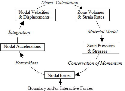
The typical series of calculations that are carried out each incremental time step (or cycle) in an element are shown schematically in Figure 3.2: Computational Cycle. Starting at the bottom of Figure 3.2: Computational Cycle the boundary and/or interactive forces are updated and combined with the forces for inner zones computed during the previous time cycle. Then, for all non-interactive nodes, the accelerations, velocities and positions are computed from the momentum equation and a further integration. From these values the new zone volumes and strain rates may be calculated. With the use of a material model together with the energy equation the zone pressures, stresses and energies may be calculated, thus providing forces for use at the start of the next integration cycle.
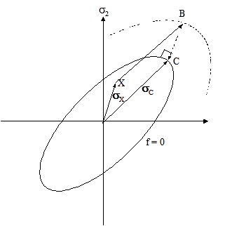
Having determined the strain rates and the volume change  the stresses can be calculated. These are then checked against the quadratic
limit criteria of equation Equation 3–29. Initially all stresses are
updated using an elastic relationship. If these stresses remain within the yield surface then
the material is assumed to have either loaded or unloaded elastically. If, however, the
resultant updated stress state lies outside of the yield surface, point B in Figure 3.3: Yield surface, steps must be taken to return the stresses normal to the
yield surface.
the stresses can be calculated. These are then checked against the quadratic
limit criteria of equation Equation 3–29. Initially all stresses are
updated using an elastic relationship. If these stresses remain within the yield surface then
the material is assumed to have either loaded or unloaded elastically. If, however, the
resultant updated stress state lies outside of the yield surface, point B in Figure 3.3: Yield surface, steps must be taken to return the stresses normal to the
yield surface.
The backward-Euler stresses are calculated as,
 | (3–41) |
where, C is the elastic stiffness matrix and from the flow rule,
 | (3–42) |
which involves the vector aC that is normal to the yield surface at the final position C. At this location the stress state satisfies the yield criteria. Except in special cases this vector aC cannot be determined from the data at point B. Hence an iterative procedure must be used.
As a first step a predictor stress state,
 is calculated using the following equation,
 | (3–43) |
where,
 | (3–44) |
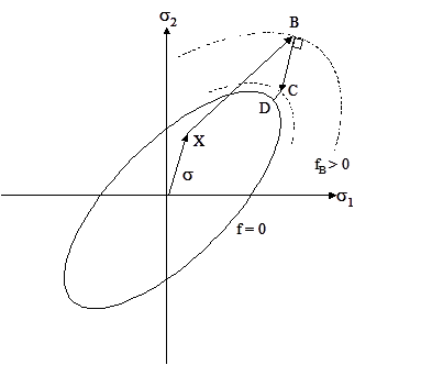
dλ here is defined so as to make the value of the yield function zero when a Taylor expansion of the yield criteria is performed about the trial point B. In general this will result in a stress state that still remains outside of the yield surface. This is because the normal at trial elastic state B is not equal to the final normal at point D (see Figure 3.4: Schematic representation of backward-Euler return algorithm). Further iterations are therefore usually required.
The stress return is achieved using a backward-Euler return algorithm and the yield function is assumed to be satisfied if the returned stress state is within 1% of the yield surface.
Once the yield function is satisfied the plastic portion of the strain increment is determined from the following,
 | (3–45) |