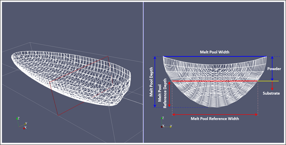
In the Additive application, we track the instantaneous melt pool along the bead length and then average the value of each dimension over the entire bead length. Output files are provided for the individual permutations, showing the full progression along the bead length, and a summary file of the average and median melt pool length, reference depth, and reference width for each permutation. From the following figure, we see that the reference depth is the entire melt pool depth minus the Layer Thickness, or the melt pool depth starting from the bottom of the first layer. Similarly, the reference width is the width at the bottom of the first layer (the start of the substrate).
It is the median result of any particular dimension you should use when interpreting your data, rather than the average result. The average will be skewed by the beginning of the bead when the melt pool is not yet stable. Let's examine the results from our example.
![]()
Individual Melt Pool Results
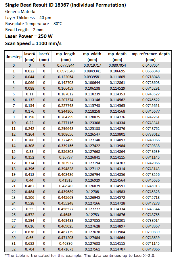
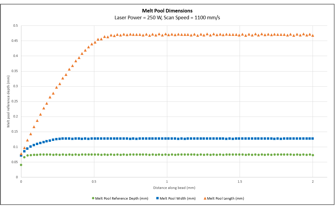
Results from an individual permutation (that is, one combination of power and speed) are shown below. A .csv file called L0_Meltpool.csv (for Layer 0) is output for each permutation. (You may find it useful to open it in Microsoft Excel and save it as an Excel table with a bit of formatting as shown here.) The timestep and distance along the bead (the mesh size) are determined internally. For this power/speed combination, we can plot melt pool dimensions against distance along the bead (laserX column) to observe when the melt pool has reached steady state. In our example, convergence is reached within 0.3 to 0.5 mm, as shown in the chart.
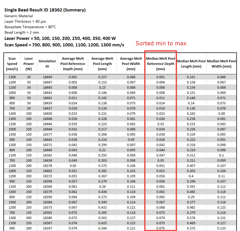
Summary Results
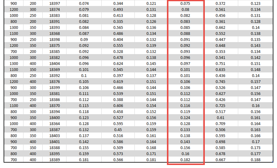
The Single Bead Summary file summarizes the melt pool characteristics for all 56 permutations. The parametric variables are listed in the left two columns; scan speed and laser power. We'll begin by sorting the data by median melt pool reference depth to see how scan speed and laser power influence melt pool depth. As a quick check of our data, for the last row with the deepest melt pool (0.182 mm median reference depth), we would expect to see the highest power and slowest scan speed combination. Indeed, our data shows the highest power (400 W) and slowest scan speed (700 mm/s) permutation from our simulation.
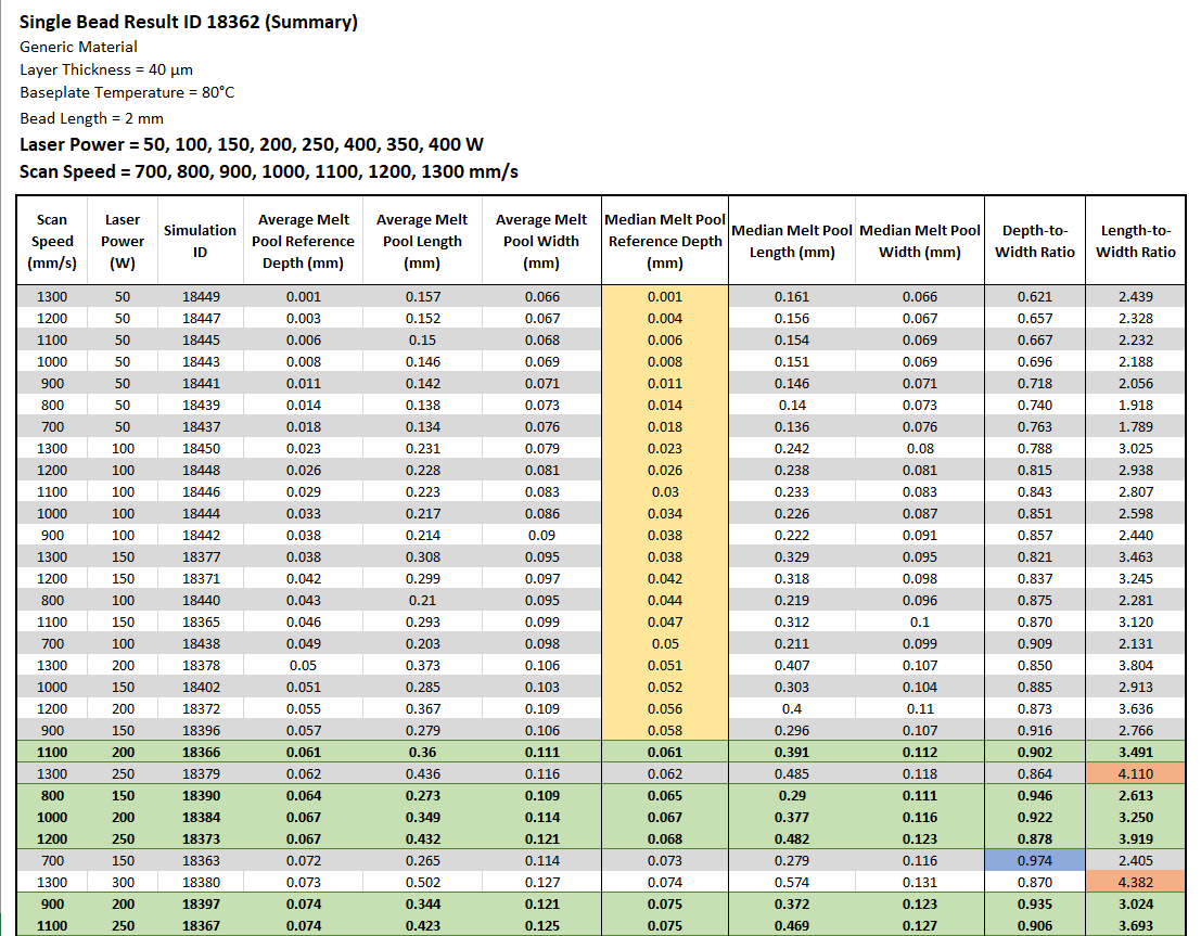
In our example simulation, we added columns in the summary table to calculate depth-to-width ratio and length-to-width ratio using the simulation data. We made the following hypothetical assumptions regarding the criteria for "good-candidate" power/speed combinations:
We want a melt pool depth that reaches at least halfway through the third layer. A penetration depth of about three layers through the thickness reduces porosity by remelting previous layers. Since our layer thickness is 40 microns (0.04 mm), that means we want a melt pool depth of at least 0.1 mm, which is a median melt pool reference depth of at least 0.06. The data that fall outside of our acceptable criteria for melt pool reference depth are shown in the yellow shaded area of the median melt pool reference depth column. These melt pools are not deep enough.
We want a depth-to-width ratio below 0.95. The data that fall outside of our acceptable criteria are shown in the blue shaded area of the depth-to-width ratio column. These melt pools are too deep.
In fact, when the melt pool becomes too large and outside of the software's acceptable range, the Additive application will error out with the following message..."
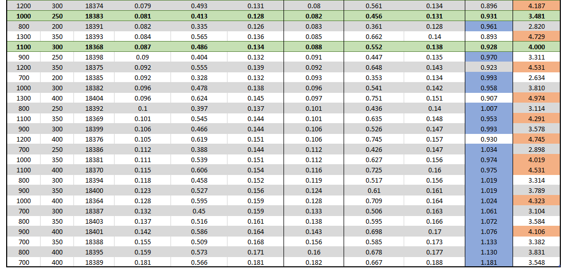
INVALID STATE: The melt pool has become too wide and deep to produce
              valid results (current width = xxx microns, current depth = xxx microns). We recommend
              you reduce the energy input by reducing Laser Power and/or increasing Scan
              Speed.
We want a length-to-width ratio below 4.0. The data that fall outside of our acceptable criteria are shown in the orange shaded area of the length-to-width ratio column. These melt pools might be too long.
Data points that meet all the good-candidate criteria above (power/speed combinations that are not in the yellow, blue, or orange shaded regions) are shown in the green shaded rows in the summary table.
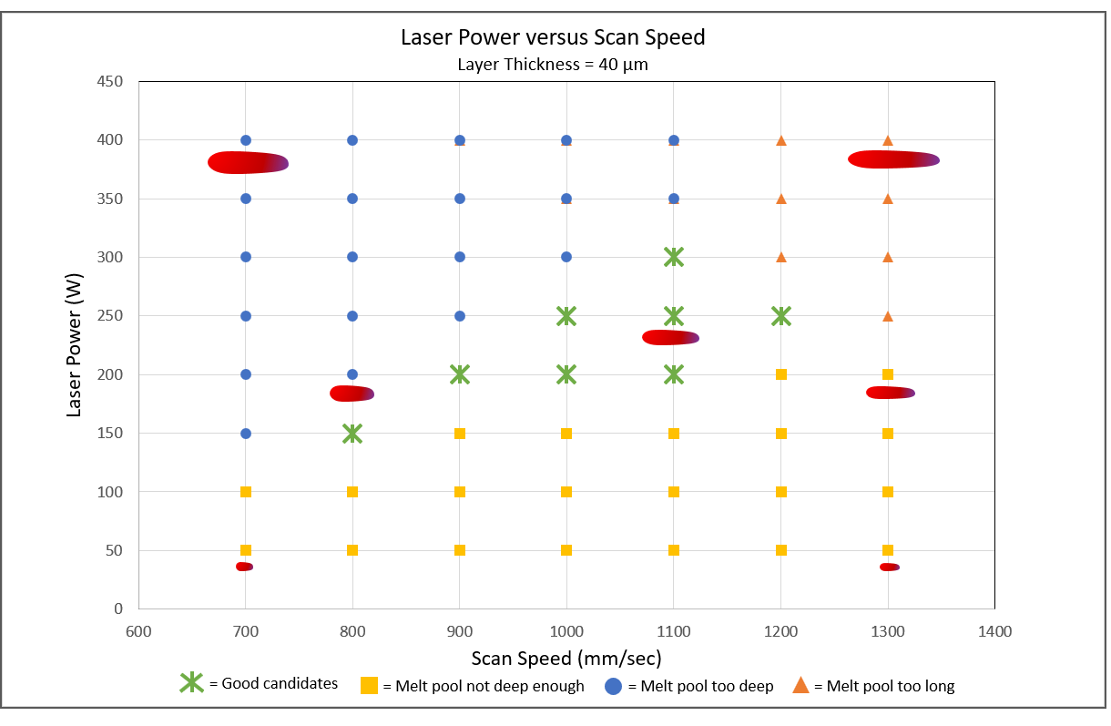
The following is a chart of all the data from the summary table shown in a power/speed process map. We can make the following observations:
The eight good-candidate power/speed combinations are shown as green stars.
Data points in yellow are the power/speed combinations that fall outside our acceptable criteria for melt pool reference depth, indicating melt pools that are not deep enough. This makes sense given that the yellow points are in a region of the map with high scan speeds and low laser power (that is, low energy density), which could contribute to lack-of-fusion porosity between the layers.
Data points in blue are the power/speed combinations that fall outside our acceptable criteria for depth-to-width ratio, indicating melt pools that are too deep. This makes sense given that the blue points are in a region of the map with low scan speeds and high laser power (that is, high energy density), which could lead to keyhole formation.
Data points in orange are the power/speed combinations that fall outside our acceptable criteria for length-to-width ratio, indicating melt pools that may be too long. This is an area of the map with the highest speeds and the highest powers, an area which has the potential for the generation of spatter and for a beading effect known as balling.
Based on median width and length data from the table, melt pool sizes ( ) are shown for a few sample points in the
chart to show relative sizes of the melt pools. Note that these are not
true scale.
) are shown for a few sample points in the
chart to show relative sizes of the melt pools. Note that these are not
true scale.
We will examine the good-candidate combinations further in a Porosity Parametric simulation.