Autospectrum

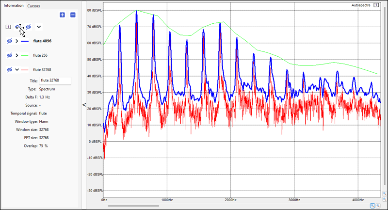
Autospectrum is a method used to estimate the power spectrum.

The principle of this method is to calculate the FFT of every slice of the analyzed signal, then to calculate the average FTT, and then to apply a normalization factor to compensate for the effect of the analysis window on the overall level of the spectrum (applying a window to a signal slice changes its level).

The autospectrum exhibits conservation of the energy. This means that summing the autospectrum (summing the magnitudes across all the frequencies) will give the same level L_eq as the original signal (L_eq is the average RMS level). This also means that the level of a tonal component (a peak in the spectrum) is given by summing the energy of the peak within its main lobe. When using FFT analysis, the energy of a pure component (peak) is often spread in the surrounding frequencies. The width and shape of this distribution depends on the FFT size and the type of the analysis window.

The formula used for the autospectrum calculation in SAS is:

Where,

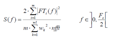
FT is the Fourier Transform of the signal (mathematical function).
m is the number of slices of the signal (determined by the overlap ratio and window size selected by the user).
wl is the window size.
w is the analysis window (of length wl samples).
nfft is the number of samples used to calculate the FFT on the windowed signal.
Fs is the sampling frequency of the analyzed signal.

Tip: The autospectrum method is better suited to the analysis of broadband components (often referred to as noise).

Note: In versions of SAS prior to 2022 R2, Autospectrum corresponds to the settings combination {Autospectrum normalization, Mean average calculation}.