


Visualizing Results
This page describes how to visualize various types of results (.xmp, .xm3, .lpf, .ies or .ldt files etc.).
Simulations results are stored in the SPEOS output files directory of the project and are available from the Speos tree.
To open a simulation result, double-click the result from Speos tree to automatically open it with the associated viewer/editor.
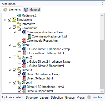
To display or hide a result in the 3D view, check or clear the result's check box.
 |
 |
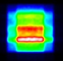
XMP Map (*.xmp)
Extended maps provide photometric or colorimetric information and measures.
XMP results are opened with the Virtual Photometric Lab.
XMP results do not appear in the 3D view when an intensity sensor with a Conoscopic orientation is used for simulation.
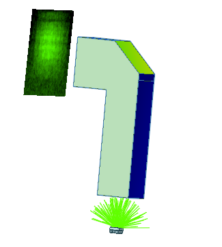
Spectral Irradiance Map (*.Irradiance.xmp)
Spectral irradiance maps are a type of extended map that provide the radiometric power or flux received by the pixels of the sensor in W/m2.
They are generated when using a Camera Sensor with an *.OPTDistortion file V1 or V2 in an Inverse Simulation.
The PNG file resulting from the simulation of the Camera Sensor using either the *.OPTDistortion file V1 or V2 is right side up as it corresponds to the post-processed image.
Spectral Exposure Map (*.Exposure.xmp) with Camera Sensor
Spectral Exposure maps are a type of extended map that provide information on the acquisition of Camera Sensors and express the data for each pixel in Joules/m²/nm.
They are generated for each Camera Sensor during a dynamic Inverse Simulation, that means:
- If the Timeline parameter is activated in the Inverse Simulation
- And at least one Camera Sensor is moving
The PNG file resulting from the simulation of the Camera Sensor using either the *.OPTDistortion file V1 or V2 is right side up as it corresponds to the post-processed image.
Spectral Exposure Map (*.Exposure.xmp) with Camera Sensor and Surface Source
Spectral Exposure maps are a type of extended map that provide information on the acquisition of Camera Sensors and express the data for each pixel in Joules/m²/nm.
They are generated for each Camera Sensor during a dynamic Inverse Simulation, that means:
- If the Timeline parameter is activated in the Inverse Simulation
- And one Surface Source is defined along with its Timeline parameters
The PNG file resulting from the simulation of the Camera Sensor using either the *.OPTDistortion file V1 or V2 is right side up as it corresponds to the post-processed image.
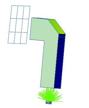
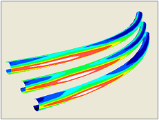
XM3 Map (*.xm3)
- spin: middle mouse button
- spin + center definition: middle mouse button when clicking on the mesh
- pan: SHIFT + middle mouse button
- zoom: CTRL + middle mouse button
XM3 maps allow to analyze light contributions on a geometry.
Ray File (*.ray)
Ray files are generated when the ray file generation is activated during a Direct Simulation.
Ray file results store all rays passing through the sensor during propagation. They can be reused to describe a light source emission.
The results are opened with the Ray File Editor.
Intensity File (*.ies, *.ldt)
Intensity files come in various formats and are created when using an Intensity Sensor in an Interactive or Direct Simulation.
Depending on the file format, the results might open with:
- Eulumdat Viewer for a *.ldt file.
- IESNA Viewer for an *.ies file.
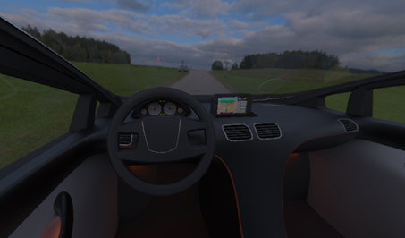
Speos360 File (*.speos360)
Speos360 files are generated when an Observer Sensor is used during simulation.
The results are opened with the Virtual Reality Lab.
HDRI File (*.hdr)
HDR images are generated at the end of an Inverse Simulation.
The results are opened with the Virtual Reality Lab.
Light Path Finder Files (*.lpf, *.lp3)
Light Path Finder files are generated when the Light Expert option is activated during a simulation.
For more information, see Light Path Finder Results.
XMP Map of Sensors Included in Light Expert Group
When a Light Expert Group has the Layer type set to Data separated by Sequence, the sequence order displayed in Virtual Photometric Lab for each sensor's XMP map changes compared to whether each sensor is included individually in a simulation.
- When a sensor is included individually in the simulation, the sequences in the Layer list are sorted by descending order of energy.
- In case of a sensor group:
- the first sensor (according to its position related to the source) sequences in the Layer list are sorted by descending order of Energy(%) values.
- all following sensors will display the exact same sequences as the first sensor.
The goal of it is in case of a Light Expert analysis of a sensors's group, when selecting a layer in one of the XMP maps, it applies the same layer to all XMP maps so that it displays the ray path of the layer. This explains why sequences of 2nd and beyond sensors may not be sorted by descending order of energy.