Creating an Inverse Simulation

The Inverse Simulation allows you to reverse the light trajectory direction. The propagation is done from the sensors to the sources. It is useful when needing to analyze optical systems where the sensors are small and the sources are diffuse.

To create an Inverse Simulation:

Make sure the Speos inputs used to define the Simulation (example: sources, geometry, sensors) are located in the same component as the simulation, or in a child component.

From the Light Simulation tab, click Inverse .
If you want the simulation to generate a Light Path Finder file, set Light Expert to True.
If you activated Light Expert, in LPF max path, you can adjust the maximum number of rays the light expert file can contain.

Note: The default value is 1e6 (1 million rays).

For more information on Light Expert analyses, refer to Light Expert.
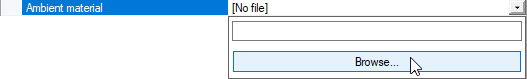
In Ambient material, browse a .material file if you want to define the environment in which the light will propagate (water, fog, smoke etc.).

The ambient material allows you to specify the media that surrounds the optical system. Including an ambient material in a simulation brings realism to the optical result.

The .material file is taken into account for simulation.

Note: If you do not have the .material file corresponding to the media you want to use for simulation, use the User Material Editor, then load it in the simulation.
If you want to consider time during the simulation, set Timeline to True.
Note: This allows dynamic objects, such as Speos Light Box Import and Camera Sensor, to move along their defined trajectories and consider different frames corresponding to the positions and orientations of these objects in simulation.
In the 3D view, click to select geometries, to select sources and to select sensors.

The selected geometry, source(s) and sensor(s) appear in their respective lists as Linked objects.
Note:
- When you include Geometric Camera Sensors, you cannot include another sensor type and you must not select a source. When you include Photometric / Colorimetric Camera Sensors, you must select a source.
- If you include an Irradiance sensor in a non-Monte-Carlo Inverse simulation, geometries are considered as absorbent.
If Light Expert is activated, the LXP check box is automatically activated for all compatible sensors whether the sensor is already listed or added afterwards. If you do not want LXP activated for a sensor, uncheck LXP for the sensor.
If some sources of your scene generate light that needs to pass through specific faces to reach the sensor (for example if you have an ambient source that needs to pass through the windshield), define out path faces/sources:
1. In the 3D view, click and select the face(s) to be considered as out path faces.
  The faces are selected and make the interface between the interior and exterior environments.
2. In the 3D view, click and select the source(s) to be considered as out sources.
  The sources are selected and are linked to the out path faces selected.
If the Optimized propagation algorithm is set to None, in Stop Conditions, define the criteria to reach for the simulation to end:

For more information on how to set Optimized propagation, refer to Monte Carlo Calculation Properties.
- To stop the simulation after a certain number of rays were sent, set On number of passes limit to True and define the number of passes.
  In case of a GPU simulation, the number of passes defined corresponds to the minimum threshold of rays received per pixel. That means while a pixel has not received this minimum number of rays, the simulation still runs.
  Note: If you activated the dispersion, this minimum threshold is multiplied by the sensor sampling. That means for a number of pass of 100 and a sampling of 13, each pixel will need to receive at least 1300 rays (the progress of the number of rays per pixel is indicated in the Simulation Progress Bar).
  In case of a CPU simulation, the number of pass, there is no minimum threshold of rays to be received per pixel, the simulation stops when the number of pass is reached.
- To stop the simulation after a certain duration, set On duration limit to True and define a duration.
  Note: If you activate both criteria, the first condition to be reached ends the simulation.
  If you select none of the criteria, the simulation ends when you stop the process.
  
  Note: If you want to adjust the Inverse Simulation advanced settings, see Adjusting Inverse Simulation settings.
If the Optimized propagation algorithm is set to Relative or Absolute, in Stop Conditions, define the Absolute stop value or Relative stop value to reach for the simulation to end.
For more information on how to set Optimized propagation, refer to Monte Carlo Calculation Properties.
If Timeline is set to True, from the Timeline section, define the Start time.

Warning: From the version 2022 R2, the Timeline Start have been improved in order to enter time values below 1ms. This change will impact your custom scripts, and will need to be modified consequently, as previous time format is no longer supported.
Preview the Meshing of the geometries before running a simulation and adjust meshing values if needed to avoid simulation or geometries errors.
In the 3D view, click Compute to launch the simulation.

Tip: To faster compute the simulation using GPU cores, click GPU Compute option .
To compute the simulation in progressive rendering, click Preview . This option opens a new window and displays the result as the simulation is running.

Preview is compatible with NVIDIA GPUs only. GPUs supported are NVIDIA A5000 or higher.

The Inverse Simulation is created along with .xmp results, an HTML report and if Light Expert is activated, a .lpf file. The .xmp result also appears in the 3D view on the sensor(s).

If Timeline is not activated and the Inverse Simulation uses a Camera sensor, only a HDRI file (*.hdr) is generated.

If Timeline is activated and a Camera sensor is moving, the Inverse Simulation is considered as dynamic and only generates a spectral exposure map for each sensor, even the static sensors. This map corresponds to the acquisition of the camera sensor and expresses the data for each pixel in Joules/m²/nm.