


Tolerancing

Once all the tolerance operands and compensators have been defined, the tolerance analysis may be performed. To perform a tolerance analysis, select Tolerancing from the Tools menu in the main program menu bar.
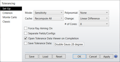
The dialog box which appears has several controls which are described below.
Set-Up tab
Mode: Four modes are supported: Sensitivity, Inverse Limit, Inverse Increment, and Skip Sensitivity.
Sensitivity mode computes the change in the criterion for each of the extreme values of the tolerances. Inverse Limit computes the value of each tolerance that will yield a criterion being equal to the value specified by the Limit parameter. The Limit parameter is only available if the mode is
Inverse Limit. Inverse mode will change the min and max values of the tolerance operands. See "Inverse sensitivity analysis" .
Inverse Increment computes the value of each tolerance that will yield a change in the criterion equal to the value specified by the Increment parameter. The Increment parameter is only available if the mode is Inverse Increment. Inverse mode will change the min and max values of the tolerance operands. For a description of how change is defined, see "Change" below. See "Inverse sensitivity analysis" .
Skip Sensitivity will bypass the sensitivity analysis and proceed to the Monte Carlo analysis.
Polynomial: The Polynomial feature has three options: None, 3-Term, and 5-Term. If either 3-Term or 5-Term is selected, the tolerance sensitivity will be determined at 4 and 6 points, respectively, spanning the tolerance perturbation range and a polynomial fit of the resulting criterion as a function of the tolerance perturbation will be computed and displayed. The 5-Term polynomial is:

where Δ is the tolerance perturbation value and P is the resulting criterion. The 3-Term polynomial omits the D and E terms. Because the polynomial fit requires evaluation of the criterion and compensators at multiple points, selecting this option increases the computation time. However, the polynomial values are cached, and once computed, can be used to greatly speed up subsequent tolerance runs with modified tolerance values.
See Cache below for details.
Cache: The cache feature can be used to greatly speed up the sensitivity and inverse sensitivity tolerance analysis, but must be used with some care. The first time the tolerance analysis is run, all the tolerances, perturbed criterion, and polynomial fit data (if any) is saved in memory. This cached data may be used to quickly generate the tolerance analysis again. If "Recompute All" is selected, the cached values are ignored, and all the tolerances are computed in full, and the new values stored in the cache. If "Recompute Changed" is selected, then only those tolerances that have been modified are recomputed. Results for unmodified tolerances are extracted from the cache rather than computed, significantly speeding up the analysis. If "Use Polynomial" is selected, than the last polynomial fit computed for each tolerance is used to quickly estimate the perturbed values. OpticStudio will automatically invalidate the cached values if any of the tolerance settings, such as criterion or Sampling, are modified. However, if any significant changes are made to the lens file itself, such as modifying surface data, the cached tolerances may be incorrect but OpticStudio is unable to detect this. Therefore, the cache feature should only be used in a single session where no changes are being made to the lens. The intention of this feature is to significantly speed up a sequence of tolerance analysis where changes are being made to the values of individual tolerances, but no other changes are being made between tolerance runs. If there is ever a doubt as to the validity of the cached data, set "Cache" to "Recompute All" and repeat the tolerance analysis. When using the cache, compensator data is not displayed (although the data presented does consider the affects of compensation), and separation by fields and configurations is not supported.
Change: Change determines how the change in the criterion and the predicted performance are computed. If Linear Difference is selected, then the change due to a tolerance is computed as

where P is the perturbed criterion and N is the nominal criterion. If Change is set to RSS Difference, the change is computed as:

where the function S(x) returns +1 if the x ≥ 0 and -1 otherwise.
Force Ray Aiming On: If the lens being toleranced is already using ray aiming, then ray aiming will be used when evaluating the tolerances. If ray aiming is not already on, then ray aiming will only be used if this box is checked. Generally, using ray aiming yields more accurate results but slower computation speed. For preliminary or rough tolerance work, leave the switch at the default "off", but for final or precise work, set the switch "on".
# CPU's: Selects the number of CPU's over which to spread the tolerance analysis task. More than 1 may be selected, even on a single CPU computer, in which case the single CPU will time share the multiple simultaneous tasks. The default is the number of processors detected by the operating system.
Separate Fields/Configs: If checked, the criterion will be computed and displayed for all field positions in all configurations individually. If unchecked, the criterion will be computed as an average over all field positions in all configurations. During inverse tolerancing, if Separate Fields/Configs is unchecked, the inverse analysis is done on the overall tolerance criterion, which is usually an average of performance over all fields in all configurations. The problem with using the average performance is that some fields or configurations may be significantly degraded by tolerance defects while other fields or configurations are not, and the average may not reveal the severity of the loss of performance at a few fields or configurations. If this option is checked, then OpticStudio computes the criterion at each field in each configuration individually, and verifies that each field meets either the Limit or Increment value. For Inverse Increment mode, OpticStudio computes the nominal performance at every field position and reduces the tolerances until the criterion at every field is degraded no more than the increment value. See "Inverse sensitivity analysis".
Open Tolerance Data Viewer on Completion: This option determines whether the Tolerance Data Viewer will open on completing the tolerance run. If the box is not checked, the data will still be available by opening the Tolerance Data Viewer manually.
Save Tolerance Data: If this box is checked, a .ZTD file containing the full tolerance data of the current run will be saved upon completion.
Criterion tab
Criterion: This control is used to specify what shall be used as the criterion for tolerancing. The options are:
RMS spot size (radius, x, or y): The best choice for systems which are not close to the diffraction limit; for example, systems with more than one wave of aberration. This is the fastest option. OpticStudio always uses a centroid reference for tolerancing.
RMS wavefront: The best choice for systems which are close to the diffraction limit; for example, systems with less than one wave of aberration. This is nearly as fast as RMS spot radius. OpticStudio always uses a centroid reference for tolerancing.
Merit Function: Uses whatever merit function has been defined for the lens. This is useful for user-defined tolerancing criterion. User-defined merit functions may also be required for systems with non-symmetric fields, or with significant surface apertures which remove rays. If the user-defined merit function is used, no boundary constraints on the compensators are automatically added to the merit function. If the merit function was generated by OpticStudio as one of the default merit functions, make sure the "Assume Axial Symmetry" option was checked OFF, see "Assume Axial Symmetry" for a discussion. Separate Fields/Configs is not supported when using this criterion.
Geometric or Diffraction MTF (average, tangential, or sagittal): The best choice for systems which require an MTF specification. If average is selected, the average of the tangential and sagittal responses is used. Diffraction based MTF tolerancing can be problematic if the tolerances are loose, because the diffraction MTF may not be computable or meaningful if the OPD errors are too large. This is especially true if the spatial frequency is high enough and the performance poor enough for the MTF to go to zero at some frequency below the frequency being analyzed. MTF is the slowest of the default criterion. The frequency at which the MTF is computed is specified in the "MTF Frequency" control.
Boresight error: Boresight error is defined as the radial chief ray coordinate traced for the on axis field divided by the effective focal length. This definition yields a measure of the angular deviation of the image. OpticStudio models boresight error by using just one BSER operand (see the Optimization chapter for details on BSER). Any element or surface decenters or tilts will tend to deviate the chief ray and increase the values of the BSER operand. Boresight error is always computed at the primary wavelength in radians. Boresight error should only be used with radially symmetric systems. Note boresight error gives no indication of image quality; it is a measure of the deviation of the axis ray.
RMS Angular radial, x, or y aberrations. This tolerance criterion is best used for afocal systems (see "Afocal Image Space"). The angular aberrations are based upon the direction cosines of the output rays.
User Script: A user script is a macro-like command file which defines the procedure to be used for alignment and evaluation of the lens during tolerancing. For details on this option, see the section "Using Tolerance Scripts". Separate Fields/Configs is not supported when using this criterion.
Limit: When using Inverse Limit mode, this control is active and is used to define the limit on the criterion for computing inverse tolerances. For example, suppose the Change is Linear Difference, Criterion is RMS Spot Radius, and the nominal RMS of a system is 0.035. If Limit is set to 0.050, then OpticStudio will compute the min and max value of each tolerance that degrades the performance to an RMS of 0.050. The Limit value must represent worse performance than the nominal system has. When using MTF as a merit, then Limit is the lower bound on MTF since lower numbers indicate worse performance. See "Inverse sensitivity analysis". The nominal value for the currently selected criterion may be computed by pressing the "Check" button adjacent to the Limit edit window.
Increment: When using Inverse Increment mode, this control is active and is used to define the limit on the change in the criterion for computing inverse tolerances. For example, suppose the Change is Linear Difference, Criterion is RMS Spot Radius, and the nominal RMS of a system is 0.035. If Increment is set to
0.01, then OpticStudio will compute the min and max value of each tolerance that degrades the performance to anRMS of 0.045. The Increment value must be positive to represent a degradation in performance. When using MTF as a merit, the Increment is still positive, and OpticStudio automatically interprets this number as a decrease in MTF from the nominal. See "Inverse sensitivity analysis". The nominal value for the currently selected criterion may be computed by pressing the "Check" button adjacent to the Increment edit window.
Sampling: Sampling is used to set how many rays are traced when computing the tolerance criterion. Higher sampling traces more rays, and gives more accurate results. However, the execution time increases. If the selected criterion is RMS spot or RMS wavefront, then the sampling value is an integer that refers to the number of rays traced along a radial arm of the pupil in the Gaussian quadrature technique (see "Selecting the pupil integration method" for a description of this technique). The number of arms is always twice the number of rays along each arm. If MTF is the selected criterion, then the sampling refers to the pupil grid size, with a sampling of 1 yielding a 32 x 32 grid, sampling of 2 yielding a 64 x 64 grid, etc. Usually, a sampling of 3 or 4 is sufficient for quality optical systems. Systems with high amounts of aberration require higher sampling than systems with low aberration. The most reliable method for determining the best sampling setting is to run the tolerance at a sampling of 3, then again for a sampling of 4. If the results change moderately, then use the higher setting. If they change substantially, check the next higher sampling setting. If the results change little, go back to the lower sampling. Setting the sampling higher than required increases computation time without increasing accuracy of the results.
MTF Frequency: If MTF is selected as the Merit, then this control is active and is used for defining the MTF frequency. MTF frequency is measured in MTF Units, see "MTF Units".
Comp: This control determines how the compensators are evaluated. "Optimize All" will use the optimization capability of OpticStudio to determine the optimum values of all defined compensators. Although optimization is accurate, it is slow to execute. There are two different optimization algorithms available, DLS and OD. If "Optimize All (DLS)" is selected, OpticStudio will execute one cycle of the Orthogonal Decent algorithm then execute the Damped Least Squares algorithm. If "Optimize All (OD)" is selected, Then the Orthogonal Descent algorithm only is used. For more information, see "Performing an optimization" . If "Paraxial Focus" is selected, only the change in paraxial back focus error is considered as a compensator; all other compensa- tors are ignored. Using Paraxial Focus is very useful for rough tolerancing, and is significantly faster than using "Optimize All". If "None" is selected, no compensation will be performed, and any defined compensators will be ignored.
Config: For multi-configuration lenses, indicates which configuration should be used for tolerancing. The selected configuration only will be considered, and the configuration number will be printed on the final report. If "All" is selected, then all configurations will be considered at once.
Fields: Generally speaking, the field definitions used for optimization and analysis are inadequate for tolerancing. for example, a rotationally symmetric lens may use field definitions of 0, 7, and 10 degrees. For tolerancing purposes, the lack of symmetry in the field definitions may cause inaccurate results when analyzing tilt or decenter tolerances. When constructing a merit function to use for tolerancing OpticStudio can use three different field settings:
Y-Symmetric: OpticStudio computes the maximum field coordinate, then defines new field points at +1.0, +0.7, 0.0, -0.7, and -1.0 times the maximum field coordinate, in the Y direction only. All X field values are set to zero. This is the default for rotationally symmetric lenses.
XY-Symmetric: Similar to Y-Symmetric, except there are 9 field points used. The 5 Y-Symmetric points are used, and -1.0, -0.7, +0.7, and +1.0 are added in the X axis direction only.
User Defined: Use whatever field definitions exist in the current lens file. This option is required when using vignetting factors, tolerancing multiple configuration lenses, or using tolerance scripts. It is also highly recommended when tolerancing non rotationally symmetric lenses or lenses with complex field weighting that user defined fields be used.
If user defined fields are used, no adjustment of the weights is performed. For the Y-Symmetric case, the center point has a weight of 2.0, all others have a weight of 1.0. For the XY-Symmetric case, the center point has a weight of 4.0, all others unity.
Cycles: This determines how rigorously OpticStudio will attempt to optimize compensator values. If set to Auto, then OpticStudio will call the optimizer in "Auto" mode, which will run the optimizer until the optimization of the compensators has converged. For rough tolerancing, a low number, such as 1, 2, or 3, may be used. If the compensators are difficult to optimize, a higher setting may increase accuracy. If too few optimization cycles are selected, then the tolerances will be pessimistic; the predicted performance will be worse than the actual performance. The "Auto" setting is the safest to use. Higher settings increase accuracy at the expense of run time. This setting is only used if Comp is set to "Optimize All".
Script: The name of the script, if using the User Script criterion. User scripts must be text files ending in the extension TSC and be in the <data>\Tolerance folder (see "Folders" ).
Status: This control is used by the tolerance algorithm to provide status messages during computation of the nominal criterion when "Check" is pressed.
Monte Carlo tab
# Monte Carlo Runs: This control is used to specify how many Monte Carlo simulations should be performed. The default setting of 20 will generate 20 random lenses which meet the tolerances specified. See the section "Monte Carlo simulations" for more details. The number of Monte Carlo runs may be set to zero, which will omit the Monte Carlo analysis from the summary report.
# Monte Carlo Save: This option is used to save a specific number of lens files generated during the Monte Carlo analysis. The value specifies the maximum number of lens files to be saved. For example, suppose 20 is selected. After the first Monte Carlo lens is generated, the lens file will be saved in the file "MC_T0001.ZMX" (depending on the file format of the original lens file). The second Monte Carlo lens file will be generated, then saved in "MC_T0002.ZMX", and so on. Only the first 20 Monte Carlo lenses will be saved (the last will be "MC_T0020.ZMX"). If fewer than 20 Monte Carlo runs were requested, then fewer than 20 lenses would be saved. Be sure you have no lens files with the names "MC_Txxxx.ZMX", as OpticStudio will overwrite these files without warning as the lenses are saved. The purpose of this feature is to allow further study on the lenses being generated by the Monte Carlo feature. Note that the file names given here assume that no File Prefix to the Monte Carlo file names was defined; see File Prefix for details.
Statistics: Choose either a Gaussian "normal" distribution, "uniform", or "parabolic" distribution. This setting is only used by the Monte Carlo analysis; see that discussion for details on the statistics mode as well as the "STAT" command which provides detailed control over the statistics model used.
File Prefix: If a prefix string is provided, then the string will be prepended to the names of the Monte Carlo files generated. For example, if the prefix string is "Fast_Doublet_" then the first Monte Carlo file saved will be file name "Fast_Doublet_MC_T0001.ZMX" (depending on the file format of the original lens file), and similar names for the remaining saved files.
Save Best and Worst Monte Carlo Files: If checked, the best and worst Monte Carlo lens files generated will be saved. The file names are "prefixMC_BEST" and "prefixMC_WORST" where "prefix" is the File Prefix string.
Overlay MC Graphics: If checked, each open analysis graphical window (such as a ray fan or MTF graph) will be updated and overlayed for each Monte Carlo generated lens. The resulting plots are useful for showing the total range of performance for the simulated lenses. Analysis graphs which do not automatically change scale and do not depend upon surface numbers are the most useful, such as MTF, MTF vs. Height, Encircled Energy, and other plots that allow a user defined fixed scale, such as ray fan plots. Plots which change scale dynamically or require a fixed range of surfaces, such as layout plots, will not work reliably and are not supported. Static, Text, and Editor windows are not updated. Overlayed graphic windows will be flagged as static after the tolerance analysis is complete. The time to compute each of the analysis graphics for each MC lens obviously will slow down the tolerance analysis.
Classic tab
Show Descriptions: If checked, a full description of the meaning of each tolerance operator will be provided in the analysis report. If unchecked, only the tolerance operator abbreviations will be listed.
Show Compensators: By default, the compensator values are not printed out during the sensitivity analysis. If this box is checked, then each compensator value will be printed along with the change in the criterion for each tolerance.
Hide All But Worst: If checked, printing of all the sensitivity data will be turned off. This is useful for decreasing the size of the output report. The "hide" check box is normally used in conjunction with the "Show worst" control.
Show worst: The "Show worst" control can be set to sort and display only some number of tolerance operands; this permits limiting the printout to the most severe tolerances only.
Output To File: If a valid file name is provided, the tolerance analysis output window text will be saved to the specified file. The path is always the same as the current lens file. Only provide a file name without a path in this box, such as OUTPUT.TXT. Leave this control blank to not save the output text.
Other buttons
There are also six buttons on the bottom of the dialog box:
Save: Save the currently selected tolerance options in a user selected file name for future use. The file ends in the extension TOP and these options may be used by other features.
Load: Restores tolerance options from a previously saved file.
Reset: Restore the settings to the default values.
OK: Performs the tolerance analysis using the current options.
Cancel: Exits the dialog box without performing the tolerance analysis, restoring the previous settings.
Apply: Saves the changed options for the session, even if Cancel is subsequently selected.
Once all of the options have been selected, press OK to begin the tolerance analysis. Details on the method of calculation are provided in the next section.
Next: