


Quick Yield

Computes the predicted Monte Carlo yield of the system using a faster, approximate calculation.
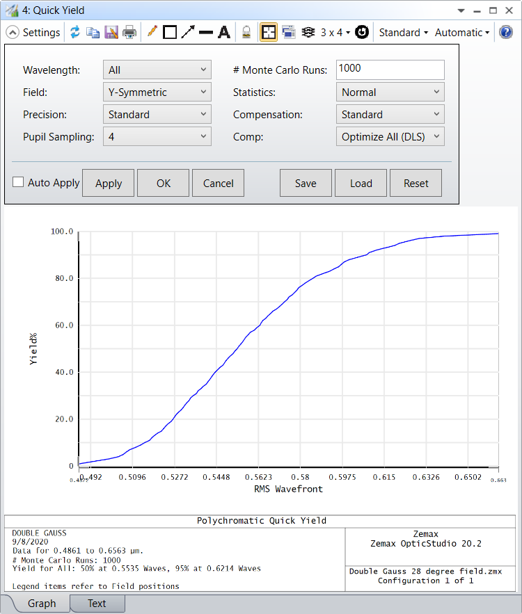
Wavelength The wavelength number used in the calculation.
Field Generally speaking, the field definitions used for optimization and analysis are inadequate for tolerancing. for example, a rotationally symmetric lens may use field definitions of 0, 7, and 10 degrees. For tolerancing purposes, the lack of symmetry in the field definitions may cause inaccurate results when analyzing tilt or decenter tolerances. When constructing a merit function to use for tolerancing OpticStudio can use three different field settings:
Y-Symmetric: OpticStudio computes the maximum field coordinate, then defines new field points at +1.0, +0.7, 0.0, -0.7, and -1.0 times the maximum field coordinate, in the Y direction only. All X field values are set to zero. This is the default for rotationally symmetric lenses.
XY-Symmetric: Similar to Y-Symmetric, except there are 9 field points used. The 5 Y-Symmetric points are used, and -1.0, -0.7, +0.7, and +1.0 are added in the X axis direction only.
User Defined: Use whatever field definitions exist in the current lens file. This option is required when using vignetting factors, tolerancing multiple configuration lenses, or using tolerance scripts. It is also highly recommended when tolerancing non rotationally symmetric lenses or lenses with complex field weighting that user defined fields be used.
If user defined fields are used, no adjustment of the weights is performed. For the Y-Symmetric case, the center point has a weight of 2.0, all others have a weight of 1.0. For the XY-Symmetric case, the center point has a weight of 4.0, all others unity.
Precision The precision level used in the approximation. The options are Standard, High, Very High. The higher the precision, the slower the calculation.
Pupil Sampling The sampling value for the number of rays traced along a radial arm of the pupil for Gaussian quadrature.
# Monte Carlo Runs The number of simulated Monte Carlo runs.
Statistics Choose either a Gaussian "normal" distribution, "uniform", or "parabolic" distribution.
Compensation The number of compensation cycles being run. Standard is 2, High is 5, Very High is 10. This analysis uses the equivalent of "Optimize All (DLS)" compensation at all times. In order to compare results to the Monte Carlo Yield, please make sure the Tolerancing tool is set up accordingly.
Comp This control determines how the compensators are evaluated. "Optimize All" will use the optimization capability of OpticStudio to determine the optimum values of all defined compensators. Although optimization is accurate, it is slow to execute. There are two different optimization algorithms available, DLS and OD. If "Optimize All (DLS)" is selected, OpticStudio will execute one cycle of the Orthogonal Decent algorithm then execute the Damped Least Squares algorithm. If "Optimize All (OD)" is selected, Then the Orthogonal Descent algorithm only is used. For more information, see "Performing an optimization" . If "Paraxial Focus" is selected, only the change in paraxial back focus error is considered as a compensator; all other compensa- tors are ignored. Using Paraxial Focus is very useful for rough tolerancing, and is significantly faster than using "Optimize All". If "None" is selected, no compensation will be performed, and any defined compensators will be ignored.
Discussion
This analysis uses sensitivity results to fit the wavefront error. The fit is extrapolated using a modified Rimmer's approach and based on this fit the Monte Carlo outcome can be reconstructed.
The exact methodology in reconstructing the Monte Carlo outcome is confidential and proprietary to ANSYS, Inc.
Quick Yield has current limitations when the compensation range is not sufficient to mitigate the Monte Carlo perturbations without reaching the compensator min or max values. In this case, the calculations will produce erroneous results. This can be avoided by increasing the compensator bounds.
Quick Yield is also limited in cases where the perturbation effects a highly non-linear. For example, when a perturbation causes significant beam clipping.
Next: