Editing Equations and Logic data

Equations and Logic Attributes store numerical data as an expression that describes how the value varies dependent on one or more parameters.

You may also see this type of Attribute also referred to as "math functional" or "EEL".

The calculation of expressions is performed in database units. The result will then be converted to the relevant display unit, if it is different.

Values are stored to a maximum of 15 significant figures.

Example: the data on applied stress vs. number of cycles to failure in this steel record is provided by the Equations and Logic Attribute Fatigue strength model (stress range):

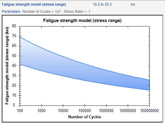
Values here are calculated using the following Fatigue Model Expression:

[A:Tensile strength] / ((1 + [P:Stress Ratio]) / (1 - [P:Stress Ratio]) + [A:Tensile strength] / (([A:Tensile strength] * (1 + [A:Elongation] / 100) - [A:Yield strength (elastic limit)]) / (log(1 + mean([A:Elongation] / 100)) - [A:Yield strength (elastic limit)] / (1000 * [A:Young's modulus])) * log(1 + mean([A:Elongation] / 100)) * (2 * [P:Number of Cycles]) ^ -0.6 + [A:Tensile strength] * (1 + [A:Elongation] / 100) * (2 * [P:Number of Cycles]) ^ (log10(mean([A:Fatigue strength at 10^7 cycles] / ([A:Tensile strength] * (1 + [A:Elongation] / 100)))) / log10(20000000))))
  1. Open the datasheet of interest and click Edit this data on the left of the Attribute name.
  2. On the Expression tab, you can see the expression that will be used to derive the data values.

    If the Attribute is configured to allow users to change the expression used, you can define a new expression or choose an alternative expression from the Expression and Domain list.

  3. Under Default Axes Preferences, you can select the parameter to use as the default x-axis.
    You can select No Free Parameter (Unbound all parameters) here and then set the bound/unbound value for each one on the Parameter Extents tab, if required.
    Select or clear the Transpose axes by default check box to transpose the graph axes. When the graph axes are transposed, the Attribute value is plotted on the x-axis, and the parameter value on the y-axis.
  4. Go to the Parameter Extents tab to specify the parameter space over which the expression is valid.

    For example, an expression to calculate strain could be defined as [ stress / Youngs Modulus ]. This would hold for values of 0 < stress < yield-stress-for-material. The parameter extent for stress can then be defined as 0 to yield-stress-for-material.

    Select Unbound to mark a parameter that is not included in the expression as applicable over all possible values. Note that parameters included in the expression must be bounded.

  5. Go to the Curves tab to add, remove, or modify the curves in the graph.
    For each curve, you can:
    • Specify the parameter values used to calculate the curve.
    • Identify it as the default curve.
    • Optionally, specify a label for the curve that will appear in the graph legend.
  6. Optional: You may be able to add metadata about the data value, such as statistical information or notes about the source of the data.
  7. Optional: You can add information about any changes that you make on the Notes tab.
  8. Click Save to save all your changes.