
Ansys SIwave™ Region-Based Simulations in HFSS 3D Layout
Simulating package/PCB layouts using Ansys SIwave™ printed circuit board (PCB) and package electromagnetics simulation software with Ansys HFSS™ regions defined around 3D structures (e.g., bondwires, irregular via transitions, BGA breakouts, et cetera), including ECAD-ECAD hierarchy (e.g., packages mounted on a PCB) and MCAD 3D components, can provide an optimal balance of accuracy and simulation time.
In a standard Ansys HFSS simulation, users designate areas in a layout as Ansys HFSS regions. During simulation, the Ansys Electronics Desktop (AEDT)TM electronics systems design platform automatically segments the selected regions into separate projects, generates virtual ports on relevant signal nets, and solves the selected regions sequentially in HFSS. Electronics Desktop then solves any geometry outside of those Ansys HFSS Regions with Ansys SIwave. As long as the points of contact (e.g., solder balls) between EDB cells lie within the selected HFSS regions, AEDT maintains simulation speed without sacrificing accuracy due to design segmentation (Refer to Hierarchical Restrictions). The resulting S-matrices from both Ansys HFSS Regions and Ansys SIwave geometry are integrated in a final circuit simulation that computes results for the entire design.
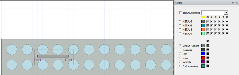
The Ansys SIwave Regions layer enables region-based simulations. Users may want to create a separate HFSS solution setup if they want to modify default HFSS settings that are used when solving HFSS regions. This HFSS simulation setup can then be associated with an Ansys SIwave region-based solution by selecting the HFSS setups/sweeps when configuring the Ansys SIwave sweep in the Edit Frequency Sweep window.
Methods of Defining HFSS Regions
There are two methods of defining HFSS regions. A standard method is used by default. An alternative method, using conformal radiation boundaries, can be selected by setting the environment variable SIWAVE_HFSS_REGION_RECESS_PORT_DISTANCE_FACTOR=<trace recess factor>. The trace recess factor can be any real value greater than 0, and defines how far, as a multiple of trace widths, the trace is recessed from the region boundary (e.g., setting SIWAVE_HFSS_REGION_RECESS_PORT_DISTANCE_FACTOR=2.5 will result in traces being recessed from the clipping extent by 2.5x the trace width).
The following table compares the two methods.
| Standard Method | Conformal Radiation Boundaries | |
| Dielectric: |
Forms a bounding box that extends 15% of width/length past the defined geometry. |
Clipped to exactly match the board outline (a conformal clip with 0% padding). |
| Radiation Boundary / HFSS Airbox: | Extends 25% past defined geometry in a bounding box. | Clipped to exactly match the board outline. |
| Signal Traces: | Signal traces that require virtual ports are slightly rerouted to ensure they hit the boundary at an orthogonal angle. |
Signal traces that require virtual ports are not clipped exactly at the region boundary; instead, their ends are moved slightly inside the boundary with no other rerouting. The distance is defined by the trace recess factor. |
HFSS Regions for Ansys SIwave Sweeps
- From the Project Tree, expand Analysis.
- Expand SIwave, if one exists.
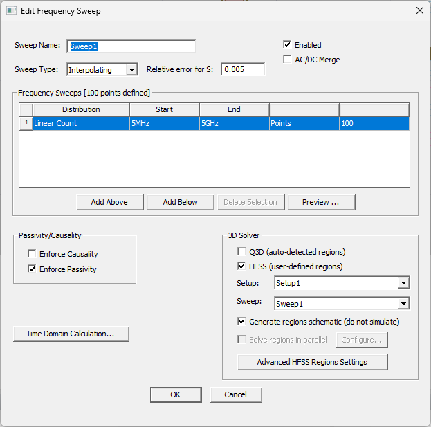
- Double-click an Ansys SIwave sweep to open the Edit Frequency Sweep window.
- From the 3D Solver area, select Q3D and/or HFSS.
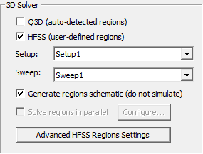
- Using the Setup and Sweep drop-down menus, select an HFSS setup and a corresponding sweep.
- If appropriate, uncheck the Generate regions schematic (do not simulate) box to activate Solve regions in parallel and Configure. Refer to Hierarchical Restrictions.
-
If appropriate, click Advanced HFSS Regions Settings to open the Advanced HFSS Regions Settings window. Use the Advanced HFSS Regions Settings window to configure simulation boundaries and trace behavior for user-defined HFSS regions in SIwave region-based simulations. These settings affect how dielectric and airbox extents are clipped, how trace ends are recessed, and how vertical padding is applied. Refer to Ansys SIwave™ Region-Based Simulations in HFSS 3D Layout.
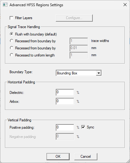
- To enable layer filtering, check the Filter Layers box. Then click Configure to open a Layer Selection window. Manually choose which signal layers are included in the HFSS region definition by checking adjacent boxes. Only selected layers will be included when defining HFSS regions. Click OK to confirm selection and close the Layer Selection window.
Note:
Filtering layers helps exclude irrelevant geometry and ensures that only signal nets intended for simulation are included in the HFSS region. Unselected layers will be excluded from simulation, and all geometry on those layers will be deleted. If all layers containing relevant signal geometry are not included, path discontinuities may result. Path discontinuity may also result if relevant GND layers are excluded (typically those immediately above and below signal layers). For example, if signal geometry exists on the Top, Bottom, and Layer 7, you should also include Layer 1 (below Top), Layer 2 (above Bottom), and Layers 6 and 8 (adjacent to Layer 7). The full set would be: Layer 1, Layer 2, Layer 6, Layer 7, Layer 8, Layer N-1, Layer N, et cetera.
- From the Signal Trace Handling area, choose how signal traces are recessed from the region boundary:
- Flush with boundary (default): Virtual ports are placed directly on the region boundary.
- Recessed from boundary by: Traces are clipped to create a gap between the virtual ports and the boundary. The recess is specified as a multiple of trace widths.
- Recessed from boundary by: Traces are clipped to create a gap between the virtual ports and the boundary. The recess is specified in millimeters.
- Recessed to uniform length: Traces are clipped so the remaining trace length is uniform across all traces in millimeters.
Note:Virtual ports must lie entirely within the region to be simulated. In the case of virtual ports generated flush to the boundary, trace routes are modified and a generous airbox is required to meet this constraint. For simulations with tight, conformal dielectric and airboxes, virtual ports must be recessed from the boundary to meet this constraint.
- From the Boundary Type drop-down menu, select the clipping method for both dielectric and airbox boundaries:
- Bounding Box: Adds horizontal and vertical padding beyond the geometry.
- Conformal: Clips exactly to the board outline (i.e., 0% padding).
- From the Horizontal Padding area, enter values for:
- Dielectric: Percentage of horizontal padding added around the dielectric region.
- Airbox: Percentage of horizontal padding added around the airbox.Note:
If Flushed with boundary (default) is selected, the boundary type is forcibly set to Bounding Box. A generous horizontal and vertical padding of approximately 15–25% is recommended. If Recessed from boundary by or Recessed to uniform length is selected, the boundary type is forcibly set to Conformal.
- From the Vertical Padding area:
- Enter values for Positive padding and Negative padding, as percentages.
- Check the Sync box to apply the same value to both directions.
Note:Vertical padding defines the extent of the simulation region above and below the board. Excessive padding may increase simulation time.
- Click OK to apply the settings or Cancel to discard changes.
Rational Interpolation
Between the actual solution frequencies, the frequency response is obtained by rational interpolation. Ansys SIwave adaptively selects the frequency points at which it computes the field solution. After a new frequency point is solved, a new interpolating fit is generated. This is compared to the interpolant on the previous step, and the maximum difference between the two is determined. If the difference exceeds the requested tolerance, then a new frequency point is selected for a solution. The interpolating sweep is complete when the difference between successive interpolants is less than the error tolerance criterion.
- From the Frequency Sweep grid, select
the method for distributing points on the Distribution option.
Select one of the following:
- Linear Count – The difference between the start frequency and the stop frequency is calculated and is divided by the number of solution points.
- Linear Step – The start frequency is incremented using the step size until the stop frequency to calculate the number of points.
- Enter the value for the minimum frequency to sweep in the Start field.
- Enter the value for a sweep maximum frequency in the Stop field.
- Specify the Points, Stepsize or Samples, depending on the Distribution option selected.
- Optionally, modify the frequency points: click Add Above, Add Below, or Delete Selection.
- To preview all the frequency points, click Preview. The Frequency List Preview window opens, showing all the points.
- Select Time Domain Calculation to export the full-wave SPICE subcircuit. The Start value changes to 0 Hz.
If there is an existing S-parameter solution, an FWS simulation can be run without needing a 0Hz or 1Hz point.
Hierarchical Restrictions
If the project contains a hierarchical layout, ensure the following:
-
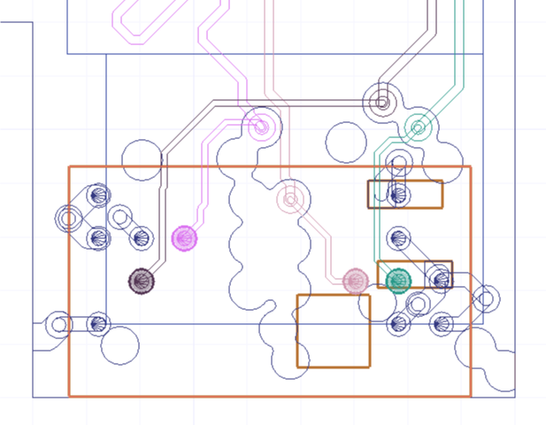
HFSS regions must surround the points of contact between both cells. Refer to Computing SYZ Solutions in HFSS 3D Layout.
-
The HFSS (user-defined regions) box is checked. If applicable, check either the Generate regions schematic (do not simulate) box or the Solve regions in parallel box. Refer to Generating a Regions Schematic in HFSS 3D Layout and Configuring a Parallel HFSS Regions Simulation in HFSS 3D Layout.
-
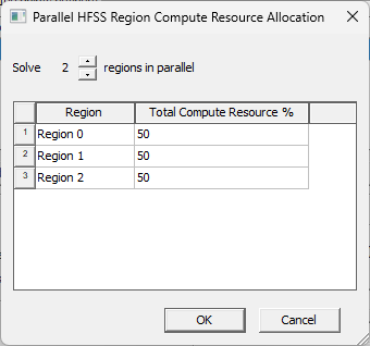
If Solve regions in parallel is checked, click Configure to open the Parallel HFSS Region Compute Resource Allocation window. Specify the number of regions to solve in parallel (e.g., 2) and allocate a percentage of total resources to each region (e.g., 50). The percentage values are converted to specific machine names, CPU counts, and memory footprints during simulation. Then click OK to close the Parallel HFSS Region Compute Resource Allocation window.
-