Using the Fields Calculator

The Fields Calculator is a very powerful tool for postprocessing. It is available for HFSS, Maxwell, Q3D, Icepak, and Mechanical solutions. While standard postprocessed results (such as S-parameters, Y or Z  matrix, animated field plots, and near and far field patterns) serve most simulation requirements, the Fields Calculator enables you to perform further computations using basic field quantities. The calculator computes derived quantities from the general electric, thermal, or displacement field solution; writes field quantities to files; locates maximum and minimum field values; and performs other operations on the field solution. Using this calculator, you can perform mathematical operations on all saved field data in the modeled geometry at a single frequency. The resulting quantities can be plotted, tabulated, or exported.

The Fields Calculator includes predefined expressions appropriate for each solver and lets you create and save additional named expressions.

To view information on a command or screen area, click over the button or screen area on the illustration below.

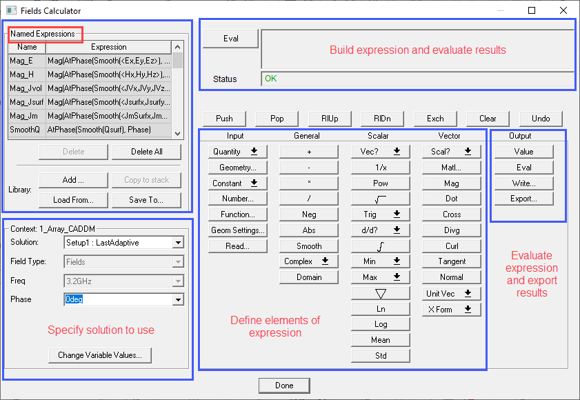
At the top-left corner of the calculator is a list of Named Expressions, which are standard or user-defined field quantities that are accessible from outside of the calculator. They can be added, copied to stack, saved to, or loaded from a library file using the buttons right beneath the list.

At the lower-left corner of the calculator is the Solution Context section, in which you can select the desired solutions, field types, frequency, and phase for the current session.

The top right of the calculator contains the Data Stack, in which calculator entries are held in stack registers. The data type in the Data Stack is denoted by its prefix abbreviation.

Immediately beneath the stack is the row of Stack Command buttons that define some basic operations for the data in the Data Stack.

The bottom half of the calculator holds the columns containing the actual calculator buttons, organized into columns, classifying them by the type of operation and the type of data upon which the operation can be performed. These columns are headed Input, General, Scalar, Vector, and Output.

At the very bottom of the calculator is the button to exit, Done. The Fields Calculator interface is discussed in detail in subsequent sections.

The calculator does not perform the computations until a value is needed or is forced for a result. This makes it more efficient, saving computing resources and time; you can do all the calculations without regard to data storage of all the calculated points of the field. It is generally easier to do all the calculations first, then plot the results.

The help for the Fields Calculator includes a "Cookbook" section that provides step-by-step examples of the following operations:

• Calculating Numerical Quantities
• Calculating Quantities for 2D (Line) Plot Outputs
• Calculating Quantities for 3D (Surface or Vector) Plot Outputs
• Calculating Quantities for 3D (Volume) Plot Outputs
• Calculating Quantities for Animated Outputs
• Creating a User Defined Named Expressions Library

Working through these examples is a good way to better understand how to use the Fields Calculator and to see what it can do for you.

Support Expression Input in Fields Calculator

For HFSS, you can create custom field quantities using algebraic expressions. For more information on this functionality, see Algebraic Mode.

Scripting Support

All calculator operations are fully scriptable. You can save the commands used in a Fields Calculator session by first clicking the Tools > Record Script to File menu and replay the same commands by clicking the Tools > Run Script menu in a later session.

Preliminary Considerations for Using the Fields Calculator

The following sections provides some consideration notes regarding use of the Postprocessor Field Calculator. Most of the statements below are fairly generalized, and may not apply to all 3D solver projects. When in doubt about the applicability of a particular consideration for a particular project, please feel free to contact your local HF Applications Engineer for further assistance.

Field Convergence and Accuracy

HFSS use finite element method (FEM) field solvers, which arrive upon a solution via adaptive meshing convergence. There are different algorithms available for determining where in each given model mesh adaptation is performed, but convergence is always evaluated by comparison of S-parameters (for driven solutions), changes in overall scattering energy (for incident wave problems) or resonant frequencies (for eigenmode solutions) from pass to pass. Because these quantities represent the results of the model as a whole, they tend to converge more rapidly than the field values. Each point in the modeled space can be said to have converged to some value. As a result, specific field quantities at each mesh point are likely to be less accurate than the overall S-parameter or eigenfrequency result of a project solution.

In order to obtain high accuracy results from calculations on field data, we recommend that you take extra precautions to assure that the model’s field data is dependable. This might include:

• Running the project to a tighter than usual convergence value.
• Seeding or manually refining the mesh in the areas to be used for calculations.
• Running parametric variations to isolate sensitivity to modeling parameters (such as adaptation frequency or circular cross-section facetization).
• Specifying expressions for output convergence.

As long as the accuracy of specific field data points to be used has been assured, the results of the Field Calculator operations should provide valuable information for your electromagnetic design tasks.

Fast Sweep and Dispersive Models

If an HFSS solution includes a Fast Frequency Sweep, the Fields Postprocessor can be tuned to display field data at any point in the frequency band swept. The specific frequency selected for viewing need not even be a precise data point at which the S-parameters were calculated. While field calculator operations may be performed at any frequency to which the Fields Postprocessor is set, fast sweep solution field data (away from the center frequency of the sweep) may not be as accurate for lossy and dispersive media, within the interior of solid-meshed finite conductors, etc. For higher accuracy under these conditions, field calculator operations should be performed on a full matrix solution completed at the desired frequency.

Because materials assigned as part of a “Perfectly Matched Layer” (PML) model termination are anisotropic and highly lossy, performing field calculations on the surface of or interior to objects designated as PMLs is not recommended.

Inputs/Excitations

Use HFSS > Fields > Edit Sources to set the field excitation appropriate to the calculation to be performed. In some cases (e.g., FSS calculations) picking the right field solution set (incident, scattered, or total) is also paramount to obtaining the intended result.

Any field calculation that has not yet been completed (such that the calculator stack still shows some form of “text” string rather than a simple numerical value) is merely a placeholder. Altering the field data loaded in the Postprocessor (by altering port excitations, changing frequency, or picking a different solution set using HFSS > Fields > Edit Sources) will result in subsequent evaluation of the placeholder to the newly loaded data. To preserve a placeholder's association to an existing data set before altering the excitation to a different data set, you should export the register stack by using the Write button. You can bring the correctly associated quantity back into the stack by using Read after you have changed the field data set selection.

Units

All units in Driven HFSS field solutions are expressed in the MKS system, regardless of drawing units. Therefore, E-mag is always in V/m, H-mag in A/m, etc. The exception is that when plotting along a geometry (e.g., along a line) the dimension along the X axis of the graph shows the position along the line in the drawing units, while the vertical (field quantity) axis will be in the MKS system.

Eigenmode Solutions

Field values in Eigenmode solutions are normalized to a peak value of 1.0, since there is no real excitation to which to scale the internal field results. If desired, you can scale the peak value to a user-selected number using the HFSS > Fields > Edit Sources menu.

Click here for scripting information related to this feature.