
Geometry, Boundaries, and Dielectric Region Support in SBR+
Boundaries Concept in SBR+
In SBR+ simulations, all geometries other than dielectric regions (discussed in Assigning a Dielectric or Conducting Material to Volumetric Region) are introduced as surfaces based on Fresnel reflection and transmission coefficients. Tables of these coefficients are either developed internally or they can be read from a user-provided file.
When a ray hits a surface, its Geometrical Optics (GO) ray fields are decomposed into surface-local transverse-electric (TE) and transverse-magnetic (TM) polarizations. Then, based on the boundary assigned to the surface and the incidence angle relative to the surface normal, the Fresnel TE and TM coefficients are obtained from the table. These are applied to the incident field to determine the GO fields of the reflected ray. If the boundary is penetrable, then Fresnel transmission coefficients are also developed from the same table and applied to determine the fields of the transmitted ray. Because the equivalent currents are developed from the total GO field at the surface, the Fresnel coefficients not only influence fields of the GO reflected and transmitted rays but also the scattered field results.
The Fresnel coefficients are defined assuming an infinitely extended plane wave and a layered planar surface that is laterally uniform and unbounded. Since, these assumptions are never satisfied - the scattering geometry is finite, rarely flat, and the boundaries change from region to region - the question arises about the suitability of Fresnel coefficients. The same objection can be made of the Physical Optics (PO) approximation applied to metallic surfaces, yet PO is a well-established approximation. This approach to handling layers is essentially a generalization of traditional PO. Provided the surface does not curve too rapidly and spans a moderate number of wavelengths, using Fresnel coefficients to determine the GO ray fields and the equivalent currents that produce the scattered field is a good approximation of the actual fields that would be measured.
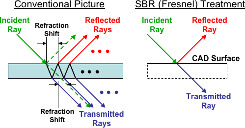
The question often arises as to whether this boundary model includes the effects of refraction, especially if the dielectric layers are electrically thick. Consider a single dielectric layer. The common picture from ray optics is that a ray enters a dielectric layer from free-space, bends due to the change in refractive index, travels through the layer, and then bends back upon leaving the layer. Hence, the exiting ray travels in the same direction as the entering ray, but it is shifted over. The reflected ray is also shifted. Moreover, there are many reflecting and transmitting rays escaping due to internal reflection within the layer. This complex picture, shown on the left in the figure below, is in sharp contrast to the simple diagram on the right that shows the rays as they are actually traced in SBR. Note that the finite thickness layer is only manifested in the reflection and transmission coefficients applied to the GO rays, not in the thin-surface CAD model itself.
In SBR, there is no spatial shift in the transmitted or reflected ray, and multiple exiting rays are not generated due to internal reflections within the layer. Again, the question arises as to whether the implementation is missing something important. The answer is that nothing is missing. The Fresnel coefficients entirely capture the impact of refraction and internal reflections, but not in the way we are used to thinking about it.
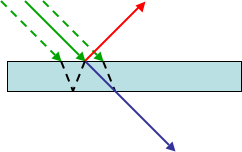
To see why, it is important to understand that while rays are traced individually, an individual ray with no neighbors has little physical meaning. In SBR+, and in GO more generally, each ray is a sampling of a larger wavefront. Individual, isolated rays do not really refract because individual, isolated rays do not even exist. The more complete picture for SBR is shown in the figure below. To preserve the refraction picture as commonly understood, one can think of the reflected or transmitted ray as continuing not the original incident ray but one of its neighbors. Likewise, the multiply reflected and transmitted rays are just continuations of other ray neighbors. The entire effect is built into the magnitudes and phases of the Fresnel coefficients. Moreover, if the simulation is applied to very thick materials and conducted over a wide frequency band, with the incident field Fourier-transformed into a narrow time-domain pulse, then the Fourier-transformed scattered fields will manifest multiple internal reflections that occur in the dielectric layer.
Perfect E Boundary
A Perfect E boundary represents a Perfect Electric Conductor (PEC) coated surface for SBR+ simulations. The configuration instructions are found in Assigning Perfect E Boundaries. In SBR+ simulations, Perfect E is a reasonable assignment for surfaces that are highly conductive at the simulation frequency, such as Copper, Aluminum, and many other high-conductivity metals at radio or microwave frequencies. Alternatively, users may consider to use a Finite Conductivity boundary in for improved accuracy.
When a ray hits a Perfect E boundary, the reflected ray field has the same magnitude as the incident ray field. The total field at the reflecting surface (incident plus reflected ray fields) has zero electric field tangent to the surface and double the incident electric field normal to surface. The opposite is true of the magnetic field (i.e., no normal component and double tangential components). Based on these constraints, and following the polarization conventions for TE and TM illustrated earlier, one can show that RTE = -1 and RTM = +1 at all incidence angles for a Perfect E boundary.
When an antenna excitation is introduced in SBR+ simulations via Huygens box, Perfect E may be assigned on its faces. When Perfect E is assigned on a face, no currents for SBR+ simulations are generated on that face. Also, presence of Perfect E indicates that the antenna has a ground plane, and the antenna can be properly installed on a platform. When Current Conformance is set to Auto, current conformance is performed only on Huygens surface at least a surface assigned to Perfect E.
Perfect H Boundary
A Perfect H boundary represents Perfect Magnetic Conductor (PMC) coated surface for SBR+ simulations. The configuration instructions are found in Assigning Perfect H Boundaries. Unlike Perfect E, Perfect H does not approximate a typical condition at a physical boundary, so it’s use is much more specialized.
When a ray hits a Perfect H boundary, the reflected ray field has the same magnitude as the incident ray field. The total field at the reflecting surface (incident plus reflected ray fields) has zero magnetic field tangent to the surface and double the incident magnetic field normal to surface. The opposite is true of the electric field (i.e., no normal component and double tangential components). Based on these constraints, and following the polarization conventions for TE and TM illustrated earlier, one can show that RTE = +1 and RTM = -1 at all incidence angles for a Perfect H boundary.
Finite Conductivity Boundary
The finite conductivity boundary is valid only if a material is classified as a PEC-like conductor. See section of PEC-like State of a Boundary below. Transmitted rays are not generated. Further instructions are found in Assigning Finite Conductivity Boundaries.
Layered Impedance Boundary
A Layered Impedance Boundary is used to model a stack of uniform layers with dielectric or conductive materials. Further instructions are found in Assigning Layered Impedance Boundaries.
The top surface of the top layer is conformal with the mesh surface, and the implied thickness of the layer is built up under the surface with respect to the incident ray. Thus, when a ray hits the boundary from above, the layers are built up below the boundary. Likewise, when a ray hits the boundary from below, the layers are built up (in the opposite direction) above the boundary.
While this is an inconsistent structural arrangement, it is convenient from a modeling perspective. The implications for users are that some thought must be given to how best to place the boundary surface in the CAD model, and this depends on which side of the surface will be predominantly illuminated by rays.
For example, consider a platform with a radome that is to be modeled with one or more dielectric layers (and no backing material). Physically, the radome has an interior surface and an exterior surface. When one is interested to predict the radiation characteristics of an antenna located behind the radome, then it is best to define the radome surfaces in the CAD model according to its interior surface. On the other hand, when one is interested to model the scattering contribution of the radome due to some source outside the radome, then it is best to define the radome surface in the CAD model according to its exterior surface. In situations where the radome is expected to be significantly illuminated by rays from both sides, the best approach is to compromise by placing the radome CAD model surface half-way between the actual radome's interior and exterior surfaces.
Layered Impedance Boundary may be configured as one- or two-sided. When configured as one-sided, the finite-thickness layers stack on top of a backing material with infinite thickness (e.g., half space). One-sided Layered Impedance is not penetrable and transmitted rays are not generated. On the other hand, when configured as two-sided, the surface is penetrable and transmitted rays are generated (see diagram above), weighted by the Fresnel transmission coefficients derived from the material and thickness properties of the layers.
Impedance Boundaries
An Impedance Boundary (IB) represents a surface with resistive and/or reactive properties. The behavior of the field at the surface and the losses generated by the currents flowing inside the surface are computed using analytical formulae. SBR+ does not actually simulate any fields inside the surface, and transmitted rays are not generated. The instructions are found in Assign Impedance Boundaries.
For an IB characterized by a surface impedance ZS, the boundary condition at the surface is Etan = ZSHtan, where Etan and Htan are the surface-tangent components of the total (incident + reflected) electric and magnetic field, respectively. Angular and frequency dependent Fresnel reflection coefficients are internally developed by the SBR+ solver from this relationship.
Fresnel (SBR+) Boundaries
Fresnel (SBR+) boundary introduces Perfect Absorber Boundary and imported Reflection – Transmission Table for SBR+ simulations. The instructions are found in Assigning (SBR+) Perfect Absorber Boundaries and Assigning (SBR+) Fresnel Table Boundaries.
Perfect Absorber
Any ray hitting a face with Perfect Absorber gets terminated, thus creating no further reflections or transmissions. However, this does not imply that there is no radiation from surface currents on perfectly absorbing surfaces. The perfect absorber still generates very strong forward scattering. This scattering is associated with the incident GO ray fields at the surface. These ray fields are converted into equivalent currents at the surface that are radiated to observation angles/points in any direction (including the backward direction); the scattered field tends to be strongest in the forward direction relative to the incident ray. At the same time, since the reflected ray has zero field strength (and therefore no reflected ray is traced), the equivalent surface currents associated with the reflected ray are also zero, so scattering in the backward half-space (relative to the incident ray) is weak.
Since we properly expect an absorbing surface to cast a shadow behind it, the strong forward scattering of the Perfect Absorber may seem unintuitive. The intuitive expectation is recovered by considering the impact on the total field rather than the scattered field. For example, consider the simplified case an antenna illuminating flat plate configured as Perfect Absorber. Behind the plate, the incident field from the antenna is strong because, by definition, the incident field is the radiation of the source in the absence of any scatterers. During SBR ray-tracing, the antenna also illuminates the perfectly absorbing plate with rays, creating a strong incident field on the plate surface. This results in a strong scattered field behind the plate relative to antenna. However, in this region behind the plate, the scattered field is 180o out-of-phase relative to the incident field of the antenna. Hence, in the “shadow” region behind the plate, the incident and scattered field destructively interfere, leaving a very weak total field. Moreover, the non-zero total field in this shadow region corresponds to fields diffracting around the edges of the perfectly absorbing plate.
Reflection-Transmission Table (.rttbl)
A Reflection – Transmission Table directly specifies Fresnel coefficients of the boundary through a reflection/transmission coefficients table file. Fresnel coefficients are based on the assumption of plane-wave incidence and reflection and represent the ratio of the reflected field to the incident field. Ray bundles can represent complex wavefronts, and each ray represents a sample of that wavefront that is assumed to be locally planar. Provided the wavefront is not too irregular, and the layers are not too thick compared to their lateral extent, the Fresnel coefficients applied in conjunction with individual rays provide a good approximation of the reflection of an arbitrary wavefront off a surface.
There are two types of the tables supported by SBR+.
- reflection coefficients
- reflection + transmission coefficients
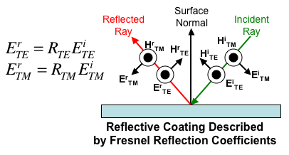
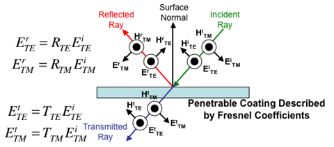
Fresnel coefficients depend on the polarization of the incident plane wave. There are two unique, orthogonal polarizations: transverse electric (TE) and transverse magnetic (TM). SBR+ adopts the convention given in the diagrams below. In this convention, PEC metal has a TE reflection coefficient of -1 and a TM reflection coefficient of +1. In general, reflection coefficients are complex quantities that depend on incident angle and frequency.
When developing tables of Fresnel coefficients for import into HFSS SBR+, it is vital to observe these polarization conventions. If the tables are generated by existing software that exports Fresnel coefficient data, then when converting the exported data into the file format expected by HFSS, special care should be taken in noting the polarization convention of that software and making sign corrections as applicable.
When a ray hits a surface, the SBR+ solver determines its incidence angle relative to the surface normal. The incident ray tube fields are decomposed into TE and TM components. SBR+ then looks up the TE and TM reflection coefficients for that angle, whether internally generated or provided by an external table as described here. These are applied to the respective incident ray field components to determine the TE and TM components of the reflected ray field.
On the other hand, penetrable boundaries, as are encountered in the case of canopies and radomes, should be described by both reflection and transmission coefficients. When creating a Layered Impedance Boundary in SBR+, if one specifies Two sided, then the solver will treat this as a penetrable and internally generate both reflection and transmission coefficients. Likewise, arbitrary boundaries that are penetrable can be entered as a table of reflection and transmission in SBR+.
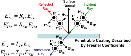
When a ray hits a penetrable boundary, it generates both a reflected ray and a transmitted ray, as shown in the diagram below, which also extends the polarization convention of the previous diagram. In the diagram below, it is intentional that the transmitted ray is shown as starting from the top of the surface, rather than the bottom. In SBR+, CAD models represent infinitely thin surfaces. The effect of layer thickness is entirely captured in the reflection and transmission coefficients. Hence, in creating a reflection + transmission table input for SBR+, it is critical to do so such that the phase reference of the transmission coefficient is the surface nearest the incident ray. That way, the transmitted ray will include the correct phase delay given that it is launched from exactly the same point as where the incident ray hit the surface.
PEC-like State of a Boundary
The PTD, UTD, and Creeping Wave enhancements in SBR+ are developed from formulations that assume perfectly conducting boundaries. However, their results remain valid for highly conducting boundaries provided they are sufficiently “PEC-like”. In addition to the Perfect E boundary, HFSS SBR+ permits deployment of these enhancements on Layered Impedance and Finite Conductivity boundaries provided their behavior is PEC-like, as determined from details of their configuration.
In the case of a Layered Impedance boundary, whether it is considered PEC-like by SBR+ depends upon the simulation frequency and the material properties of its exposed layer (the first layer in the stack.) The following table illustrates the frequency dependence for several typical metals. For example, if the exposed boundary layer is Copper and 30-μm thick, then the entire Layered Impedance boundary stack will be considered PEC-like between fmin = 192 MHz and fmax= 735 GHz. The 192-MHz lower bound is not explicitly shown in the table but is consistent with the Minimum Thickness columns for 10 MHz and 1 GHz. For simulation frequency sweeps residing within this band, wedges with this top-layer will be considered PEC-like and therefore eligible for deployment of PTD and UTD. However, if the frequency sweep partially or completely falls outside of this band, then the same wedge will ineligible. To prevent discontinuous sweep results, HFSS SBR+ will not switch on PTD, UTD, or Creeping Wave mid-sweep if the sweep crosses one of these frequency boundaries.
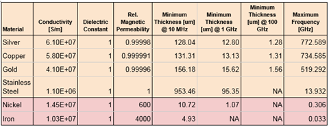
For a top-layer coating to be PEC-like, several conditions must be met, and the above table is developed from these conditions. The top layer must have free-space electric permittivity (εr = 1) and lossless magnetic permeability (Im{μr} = 0). In addition, the dielectric layer must possess the very high conductivity (σ) of a metal. Furthermore, the thickness of the top-layer coating must be greater than 2π skin depths δ=1/√(πf σμ) as computed at the lower bound of the frequency sweep. Increasing the layer thickness or its conductivity lowers the minimum frequency (fmin) at which the layer exhibits good PEC properties. Because of this skin depth requirement, additional layers do not change the PEC-like status of a Layered Impedance boundary. Likewise, whether the Layered Impedance boundary is One-sided or Two-sided makes no difference.
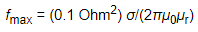
The maximum frequency fmax at which the coating is deemed PEC-like increases with the top layer’s conductivity σ and decreases with its relative magnetic permeability μr. In HFSS SBR+, fmax is computed as
Assigning a Dielectric or Conducting Material to a Volumetric Region
For a discussion, see Assigning a Dielectric or Conducting Material to Volumetric Region.