Assigning (SBR+) Fresnel Table Boundaries

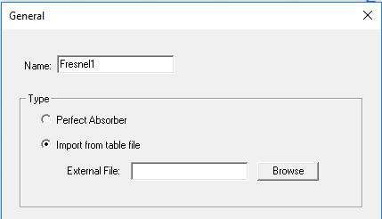
The Assign Boundary>Fresnel (SBR+) command allows you to specify either a perfect absorber or to import a Fresnel table file that describes reflection and transmission coefficients.

Fresnel coefficients are based on the assumption of plane-wave incidence and reflection and represent the ratio of the reflected field to the incident field. Ray bundles can represent complex wavefronts, and each ray represents a sample of that wavefront that is assumed to be locally planar. Provided that the wavefront is not too irregular, and the coatings are not too thick compared to their lateral extent, the Fresnel coefficients applied in conjunction with individual rays provide a good approximation of the reflection of an arbitrary wavefront off a surface

When an SBR+ boundary is configured as an Impedance Boundary or a Layered Impedance boundary, a table of Fresnel coefficients is internally generated for use during the SBR+ ray-tracing simulation. The Fresnel (SBR+) Import from table file option lets you directly load the Fresnel tables from an external file. You can develop these from a number of sources, including analytic formulas, specialized codes for simulating the boundary (e.g., HFSS for simulating a frequency selective surface), or measurements. Two types of boundary tables are supported:

• reflection coefficients
• reflection + transmission coefficients

Tables of reflection + transmission coefficients are explained later.

Fresnel coefficients depend on the polarization of the incident plane wave. There are two unique, orthogonal polarizations: transverse electric (TE) and transverse magnetic (TM). HFSS-SBR+ adopts the convention given in the diagram below. In this convention, PEC metal has a TE reflection coefficient of -1 and a TM reflection coefficient of +1. In general, reflection coefficients are complex quantities that depend on incident angle and frequency

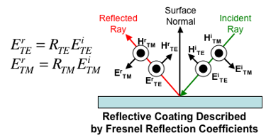
When a ray hits a surface, the solver determines its incidence angle relative to the surface normal. The incident ray tube fields are decomposed into TE and TM components. The solver then looks up the TE and TM reflection coefficients for that angle, whether internally generated or provided by an external table as described here. These are applied to the respective incident ray field components to determine the TE and TM components of the reflected ray field. This, in turn, influences the surface currents and scattered fields generated at the current bounce and subsequent bounces.

Fresnel Reflection Table File Format

The Fresnel reflection table file format is documented in the header comments in the example below. This first example is for a table defined at a single frequency, which means it will be used at all frequencies during a simulation. A multi-frequency example is provided later for a reflection/transmission table, but since their formats are nearly identical, the same encoding can be used for a reflection-only table

# Reflection table file.

# Blank lines and lines beginning with are ignored.

# The following key is critical in distinguishing between a reflection table and a reflection/transmission table.

ReflTab1e

# Incident angle, theta, is measured from the normal to the surface .

# In the table, theta is assumed to vary from C (head-on) to 90 deg (grazing) .

#The density cf angular sampling is specified by the number cf theta steps.

# In this example, there is a sample every 1 deg.

# <num theta step> number of theta points - 1

90

# Frequency domain

# Mono freq. table for 1.000000 GHz data type

# <freq_domain_type> = { MonoFreq, Multi Freq}

MonoFreq

# Data section follows. Frequency loops within theta.

# <rte_rl> <rte_im> <rtm_rl> <rtm_im>

-3.81966e-01 0.00000e+00 3.81966e-01 0.00000e+00

-3.82C18e-01 0.00000e+00 3.81914e-01 0.00000e+00

-3.82174e-01 0.00000e+00 3.81758e-01 0.00000e+00

-3.82435e-01 0.00000e+00 3.81497e-01 0.00000e+00

-3.82799e-01 0.00000e+00 3.81132e-01 0.00000e+00

-3.83269e-01 0.00000e+00 3.80662e-01 0.00000e+00

-3.83843e-01 0.00000e+00 3.80086e-01 0.00000e+00

-3.84523e-01 0.00000e+OC 3.79403e-01 0.00000e+00

-3.8S3C9e-01 0.00000e+0C 3.78613e-01 0.00000e+00

-3.86201e-01 0.00000e+0C 3.77715e-01 0.00000oe+00

-3.87200e-01 0.00000e+0C 3.76708e-01 0.00000e+00

:

:

-9.16560e-01 0.00000e+00 -6.42464e-01 0.00000e+00

-9.32634e-01 0.00000e+00 -7.03164e-01 0.00000e+00

-9.49016e-01 0.00000e+00 -7.68667e-01 0.00000e+00

-9.65704e-01 0.00000e+00 -8.39528e-01 0.00000e+00

-9.82699e-01 0.00000e+00 -9.16389e-01 0.00000e+00

-9.99900e-10 0.00000e+O0 -9.99500e-01 0.00000e+00

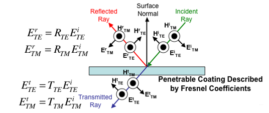
Penetrable boundaries, as are encountered in the case of canopies and radomes, should be described by both reflection and transmission coefficients. Likewise, arbitrary boundaries that are penetrable can be entered as a table.

When a ray hits a penetrable coatings, it generates both a reflected ray and a transmitted ray, as shown in the diagram below, which also extends the polarization convention of the previous diagram. In the diagram below, it is intentional that the transmitted ray is shown as starting from the top of the surface, rather than the bottom. In the modeler, CAD models can represent infinitely thin surfaces. The effect of boundary thickness is entirely captured in the reflection and transmission coefficients. Hence, in creating a reflection + transmission table input, it is critical to do so such that the phase reference of the transmission coefficient is the surface nearest the incident ray. That way, the transmitted ray will include the correct phase delay given that it is launched from exactly the same point as where the incident ray hits the surface

The following example reflection + transmission table is very similar in structure to the reflection-only table. The only difference is that each line in the table has four extra numbers to represent the complex TE and TM transmission coefficients. This particular example also shows how to define a frequency dependent table of coefficients

# EMA3D native format reflection/transmission table file

# The following key is critical in distinguishing between a reflection table

# and a reflection/ transmission table.

RTTable

# <num theta step> = number of points-1

90

# Frequency domain

# In this example, the frequency samples are from 0.5 to 4 GHz in 20MHz steps

# MultiFreq <freq_start_ghz> <freq_stop_ghz> <num_freq_steps>

MultiFreg 0.5000000 4.000000 175

# Data section follows. Frequency loops within theta

# <rte_rl> <rte_im> <rtm_rl> <rtm_im> <tte_rl> <tte_im> <ttm_rl> <ttm_im>

-6.23449e-01 1.00978e-04 6.23449e-01 -1.00978e-04 -5.88718e-01 -3.66763e-01 -5.88018e-01 -3.66763e-01

-6.12741e-01 7.99650e-02 6.12741e-01 -7,99650e-02 -6.13162e-01 -3.29510e-01 -6.13162e-01 -3.29510e-01

-5.78215e-01 1.54566e-01 5.78215e-01 -1.54566e-01 -6.44759e-01 -2.91524e-01 -6.44759e-01 -2.91524e-01

:

:

-9.99927e-01 2.21130e-05 -9.99629e-01 9.58350e-05 -1.85062e-05 -7.37198e-05 -1.07270e-04 -3.64781e-04

-9.99920e-01 2.99358e-05 -9.99596e-01 1.33667e-04 -2.89748e-05 -7.33898e-05 -1.59538e-04 -3.61020e-04