
Plotting Spectral Domain Data
Follow this procedure to plot spectral domain data from a transient simulation in the Reporter:
-
Open the Report dialog box. The following dialog box appears.
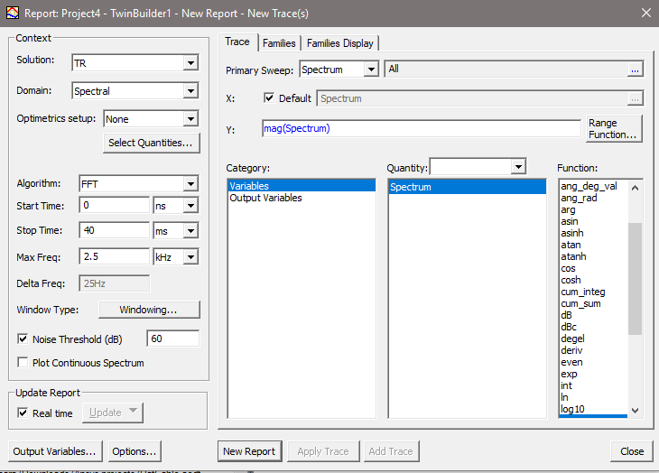
- Select the desired transient solution and set the Domain to Spectral in the Context area.
- Set the Start Time and Stop Time as desired to avoid circuit startup artifacts or late time data.
- Max Freq sets the maximum frequency for spectral analysis and plotting.
- Select the Plot Continuous Spectrum check box for a continuously plotted spectrum; clear the check box for a discrete spectrum.
-
You can toggle a Noise threshold using the check box (default value is 60 dB). This setting filters out data that is more than the specified amount below the maximum magnitude.
- To control advanced settings such as Window Type and Kaiser Param, click Windowing to open the dialog box.
Delta Freq is supplied as 1/T0 Hz, T0 = Stop Time - Start Time.
The Algorithm drop-down menu contains 3 options: Fourier Integration (FI), FFT, and Fourier Transform.
Fourier Integration and FFT both provide Fourier Series (or Fourier Coefficients) of the transient signal with DFT, where periodicity is implicitly assumed and the period is defined as T0 = Stop Time - Start Time.
Fourier Integration computes Fourier series by numerically integrating the input waveform from its transient simulation. The sampled waveform may not be on a set of evenly spaced time points. Fourier Integration is much slower compared with FFT, but it can be more accurate since it preserves the shape of underlying waveform without re-sampling.
The FFT algorithm re-samples the input waveform by interpolating to evenly spaced time points. It uses the FFTW library that is publicly available and whose computational complexity is

where N is the sample size after re-sampling and N = 2 *#Harmonics +1, where #Harmonics = Max Freq/Delta Freq.
Based on the Nyquist-Shannon Theorem or Sampling Theorem, the sampling rate should be at least twice the bandwidth of the signal to avoid aliasing.
Spectral plots based on Fourier Integration and FFT are single-sided with magnitudes of non-zero harmonics doubled because the negative frequency components are folded to the positive side.
Fourier Transform (FT) provides the Fourier transform of a signal defined in [Start Time, Stop Time] by leveraging the FFT algorithm. The Fourier transform of a time limited signal f(t) in [0, T0] is

The Fourier series of a periodic signal that is equal to f(t) in [0, T0] and with period T0 is

Hence,

In other words, the Fourier series of f(t) based on FFT can be multiplied by T0 in order to get the Fourier Transform of f(t) at sampled frequencies n/T0.
Spectral plots based on Fourier Transform only show the positive frequency side.
- Windowing functions cause the FFT of
the signal to have non-zero values away from w.
Each window function trades off the ability to resolve comparable signals
and frequencies versus the ability to resolve signals of different strengths
and frequencies. You can apply a window to the transient data to help
resolve closely spaced harmonics and to reduce spectral leakage due
to the finite nature of the time signal. Choose the Window
Type to apply to the data from the following list:
Window Function
Preferred Use
Rectangular (default)
A low dynamic range function offering good resolution for signals of comparable strength. Poor when signals have very different amplitudes. w(n)=1.
Bartlett
A high dynamic range function, with lower resolution, designed for wide band applications.
Blackman
A high dynamic range function, with lower resolution, designed for wide band applications.
Hamming
A moderate dynamic range function, designed for narrow band applications.
Hanning
A moderate dynamic range function, designed for narrow band applications.
Kaiser
Selecting the Kaiser plot also enables the Kaiser Param field to specify an associated Kaiser parameter. The larger the Kaiser parameter, the wider the window. The parameter controls the trade-off between width of the central lobe and the area of the side lobes.
Welch
This approach divides the spectrum into overlapping periodogram bins in order to more accurately depict data away from the center of the signal.
Weber
Lanzcos
The Lanczos window offers a windowed form of the infinite sinc filter, providing the central lobe of a horizontally-stretched sinc, sinc(x/a) for -a = x = a.
- If desired, select the Adjust
Coherent Gain check box, so that the signal levels are adjusted (based
on the window type) as if no window were used. When non-rectangular windows
are used, the window changes the power level of the signal.
This is known as the “coherent gain” or “processing loss” of the window.
Note:
Fourier Integration may be slightly more accurate than FFT, but can be much slower, requiring a long time to create results.
- When finished, click OK to save the settings.
For more information about the use of windows in harmonic analysis see: F.J. Harris, “On the Use of Windows for Harmonic Analysis with the Discrete Fourier Transform,” pp. 51-83, Proc. IEEE, vol. 66, no. 1, Jan 1978.