
X-Parameter Technical Notes
X-parameters are a superset of the frequency-dependent S-parameters. X-parameters are intended to model a device that generates a nonlinear response to an input whose energy is concentrated at one or a few fundamental frequencies. The response at each port consists of signals at the harmonics or the fundamental, or at the sums and differences of the harmonic frequencies of the fundamentals when more than one is present. The treatment of X-parameter models depends on the principle of harmonic superposition—the idea the harmonics are small in magnitude relative to the fundamental signal, and thus the harmonics can be superimposed linearly.
The X-parameter solver combines large-signal and small-signal models. In systems with nonlinear components, large-signal AC magnitudes can affect the operating point; small-signal contributors can be modeled accurately by linearizing the circuit around an operating point. The X-parameter solver calculates the Large-Scale Operating Point (LSOP) based on the large-signal contributors. The small-signal harmonic contributions are obtained by linearizing the system around the LSOP.
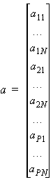
Let a be the vector of complex incident wave amplitudes to the device. Each element of the vector is indexed by port (1 to P) and harmonic (1 to N).
(1)
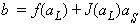
Vector b is a similarly indexed vector of scattered wave amplitudes. The vector b is a nonlinear complex function of a:
(2)
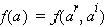
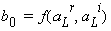
From the situation represented by an X-parameter element, vector a is composed of one or a few large signals and several small-signal harmonics:
(3)
where the vector aL contains the complex amplitudes of the large signals and zeros instead of the small-signal amplitudes. Similarly, the vector aS contains the complex amplitudes of the small signals and zeros instead of the large-signal amplitudes.
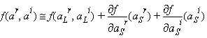
If the a inputs are real, you could approximate b as:
(4)
where J(aL) is a Jacobian matrix of the derivatives of f at a = aL with respect to the small-signals aS.
But a and b are complex, so a different formulation is appropriate.
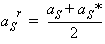
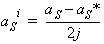
Start by splitting a into its real and imaginary parts:
(5)
where , and the superscripts r and i denote the real
and imaginary parts of a,
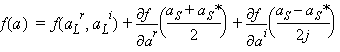
not exponents. Consider f
to be a function of two real vectors:
, and the superscripts r and i denote the real
and imaginary parts of a,
not exponents. Consider f
to be a function of two real vectors:
(6)
Then, linearizing f around the LSOP, you have:
(7)
Use the following identities to rewrite (7) in terms of aS and its complex conjugate aS*:
(8)
(9)
Substituting (8) and (9) into (7), obtaining:
(10)
Rearranging the terms involvingaS and its complex conjugate aS*:
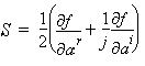
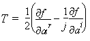
(11)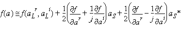
Further simplify equation (11) to show the parallels with equation (4). Let:
(12)
(13)
(14)
The complex equivalent of equation (4) is the formula for calculating the response from a set of X-parameter data and incident waves:
(15)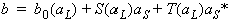
In words, b0 is a function of the large-signal inputs, or more generally, of the LSOP, while S(aL) and T(aL) are matrices that represent the linearization of the small signal harmonics around the LSOP. The complex conjugate aS* is required to account for the phase differences between the harmonic components and the large signals.
When ||b0|| = 0, T=0and b =S(a). Thus, X-parameters are a superset of S-parameters.
For each fundamental there is at least one large signal, and the LSOP includes just the absolute value of this signal. The dependence on phase of the large signal is determined on the time-invariance of the system. This dependence is captured by the use of three matrices, Pb0, PS, and PT, the entries of which are all the form ejqf, with q an integer and f the phase of aL:
(16)
Using these matrices, the dependence of b0, S, and T on aL is written as:
(17)
(18)
(19)
The LSOP can also depend on independent variables supplied in the X-parameter file. The independent variables include biasing and load conditions (See Independent Variables for X-Parameters). Then, b0, S, and T all depend on the independent variables that are used when the X-parameter data file was generated:
(20)
(21)
(22)
where xis a vector of the M independent variables
(23)
DC Equations
Equation (15) relates the scattered wave amplitudes to the incident wave amplitudes, at the fundamental frequency and at higher harmonics. However, nonlinear devices typically exhibit some degree of rectification, which means that even when the input is a single tone, the output includes a DC component.
There are two options for modeling the DC response. The X-parameter model approximates either the DC voltage at a port given the current going into it, or the DC current at a port given the voltage across it. From the first case, the port is designated as an IDC port, and this is chosen when the port is to be biased by an external current source. From the second case, the port is designated as a VDC port, and this is chosen when the port is to be biased by an external voltage source.
For both cases, follow a procedure similar to that leading to equation (15), except the functions to be approximated—either the DC currents, iDC, or the DC voltages, vDC—are real-valued.
For the IDC ports,
(24)
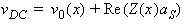
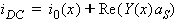
where vDC is a vector of the approximate DC voltages at all IDC ports. The vector v0(x) denotes the DC voltages at the LSOP, and the harmonic impedance matrix Z(x) relates the small-signal amplitudes at all harmonics to the DC voltages. The LSOP must include the DC currents at all the IDC ports. For the VDC ports,
(25)
where iDC is a vector of the approximate DC currents at all VDC ports. The vector i0(x) denotes the DC currents at the LSOP, and the harmonic admittance matrix Y(x) relates the small-signal amplitudes at all harmonics to the DC currents. The LSOP must include the DC voltages at all the VDC ports.
What should be written is (24) and (25) in the same form as (15), but they can be written more succinctly as:
(26)
and
(27)
which also make it clear that vDC and iDC are real.