
Fields Report
The following display types are available for fields reports in Mechanical – Structural solutions:
- 2D (Rectangular) Plot
- Stacked Plot
- Data Table
- 3D Plot
- 2D Contour Plot
In this topic, we will focus on the display types that are most likely to be used for structural reports (specifically 2D plots, Stacked plots, and Data Tables). The procedure for creating other types of plots is similar. The subtopic, Creating a Fields Report, details how to generate plots and data tables of structural fields results.
In order to create a fields report of the predefined structural results, an arc, line, or series of straight and/or curved polyline segments is needed. You can draw the line segments manually or select edges of your model and convert them to line objects. Then, specify this polyline geometry as the path along which the predefined thermal result values will be calculated and plotted.
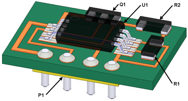
For example, the following image is a sample thermal stress analysis model. It consists of a printed circuit board (PCB), pin header, integrated circuit (IC), transistor, two resistors, and the solder used to connect all of the parts to the PCB traces:
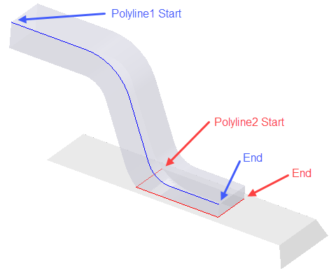
Two multi-segment polylines have been drawn, which are used to define paths for plotting the equivalent stresses along edges of interest. Polyline1 is drawn along the edges of Pin 5 of the IC. Polyline2 is drawn along three edges where the top of the solder intersects Pin 5:
- Whether you draw the polyline before or after running the solution, it's a good idea to create it as a non-model part. However, the solver will ignore line and sheet objects even if the Model option is selected in the object properties. If you create a polyline after solving, you will be prompted to create a non-model object, or the solution results will be invalidated.
- For the preceding example, the points defining the arc segments along Polyline1 are drawn slightly below the curved faces and edges of Pin 5 (about 0.005 mm). When curved object faces are discretized into a mesh, they become faceted. A pure arc segment would not pass through the elements generated along the corresponding model edges, leaving gaps in any plotted or tabulated results. Moving the curve slightly inward prevents any gaps in the output.
The available predefined structural results are listed and described under Fields Report in the Results (Structural) topic. Examples of 2D plots, Stacked plots, and Data Tables follow:
- 2D (Rectangular) Plot: This type of plot can contain one trace or multiple traces, each of which is plotted within the same Cartesian grid.
- Stacked Rectangular Plot: This type of plot is intended for multiple traces. Unlike the 2D plot previously described, this type puts every individual trace in a separate Cartesian grid stacked vertically. The X scale is shared by all traces, but the Y scale is adjusted to suit each individual trace.
- Data Table: Tabulation of any of the available fields report results as an alternative to a plotted curve.
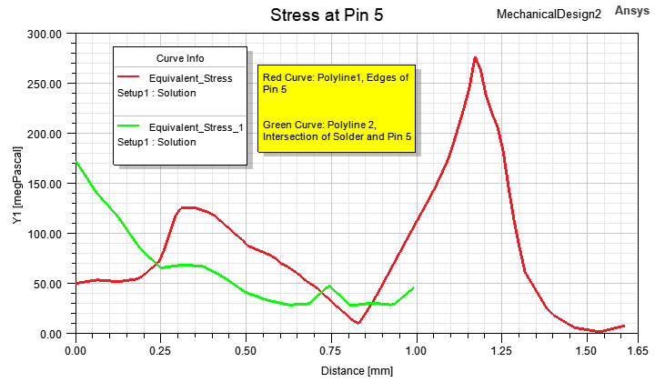
The following image shows the Equivalent_Stress vs. Distance 2D (rectangular) plot based on the preceding model and polylines example. A note has been added to identify which curve corresponds to which polyline:
As with the 2D plot, you must create a polyline object along which the predefined structural result values will be calculated and plotted.
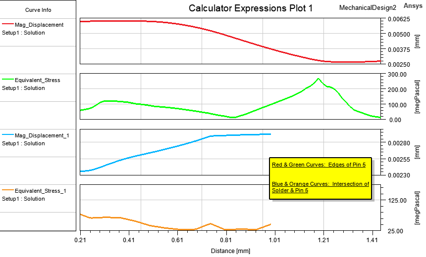
The following image is an example of a four-curve stacked rectangular plot from the same model. The top trace is the Mag_Displacement along Polyline1 (the edges of Pin 5), and the second trace is the Equivalent_Stress along the same polyline. The third trace is the Mag_Displacement along Polyline2 (the intersection of the solder and Pin 5), and the bottom trace is the Equivalent_Stress along the same polyline. For all traces, the X axis is the distance along the polylines:
The example that follows lists the Equivalent_Stress and Mag_Displacement results versus the distance along Polyline1 and Polyline2 of the same example model. The results are staggered between columns two and three (Polyline1) and four and five (Polyline2) because the Distance calculation points differ between the two lines:
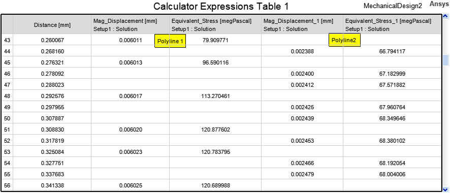
In this case, you would click and drag the scroll bar on the right vertically to see all 101 data points that were tabulated for each polyline.