Using the Hysteresis Model-Based Demagnetization/Magnetization Approach

(Transient Solver Only)

Currently, demagnetization is modeled based on single demagnetization curve in the second quadrant, possibly extended to the third quadrant in the user-specified direction. Hysteresis-based demagnetization is able to consider magnetization and demagnetization behavior at the same time in all directions, not just user-specified initial direction.

To enable hysteresis model-based demagnetization, and set the Demagnetization/Magnetization computations for source designs:

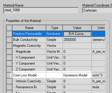
• Define the hysteresis loop by inputting the descending branch of a hysteresis loop (not supported by defining Hysteresis Model under Core Loss Model).

• Set the initial demagnetizing direction for the starting point on the hysteresis loop by setting the direction in the field for the Unit Vector input of Magnetic Coercivity on the panel of View/Edit Material during material setup. (The initial value is inherently described by the point (Hc = 0 and B = Br).

If a problem setting does not satisfy the above two conditions at the same time, the transient solver will use the “classic” approach to simulate demagnetization process if possible. Note that the valid descending branch of a hysteresis loop should be input with the same absolute values (H and B) for the 1st point and the last point. This modeling approach is not supported for TDM since the modeling of hard hysteresis material cannot be supported by Time decomposition Method (TDM).

Using the Hysteresis Model-Based Magnetization Approach

(Transient Solver Only)

With the introduction of vector hysteresis modeling capability in the transient solver, it is now possible to simulate the hysteresis model-based magnetization process if a user defines a normal nonlinear BH curve in the 1st quadrant together with the input of Hc (or additional Br for better accuracy of hysteresis loop construction) by selecting Hysteresis Model under Core Loss Model for the material.

In such a case, magnetization is always considered as isotropic magnetization, that is, magnetization direction is determined by the orientation of the computed field. If a user defines only a normal nonlinear BH curve in the 1st quadrant without defining the Hysteresis model, the transient solver will use the “classic” approach to simulate magnetization process.

Classic Magnetization Approach

Using the classic magnetization approach, if the geometry in the source and target designs is the same, Maxwell maps the computed magnetization data element–by–element. However, the geometry in the source and target designs need not be identical, in which case the geometries in the two designs will be mapped by the solver using the object name. For example, magnetization data on “Box1” in the source design will be applied to the object called “Box1” in the target design. The user must ensure that the source and target object names are identical. The source design will compute magnetization data on the selected objects, while the target design will use the dynamic data in its simulation.

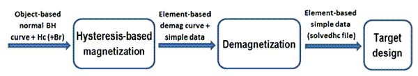
Hysteresis Model-Based Magnetization Approach

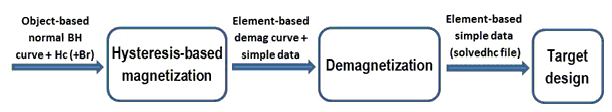
Using the hysteresis model-based magnetization approach, after the completion of the last time step before stop, the hysteresis model for each element will generate the element-based demagnetization curve originated at the last operating point. As a result, the output from the magnetization modeling process is an element-based demagnetization curve, rather than a constant. Consequently, an additional demagnetization process is required based on the element-based demagnetization curve. In this approach, use of the same mesh between the source and the two target designs is required due to the use of the element-based demagnetization curve as the output of magnetization simulation.

Design Criteria

• The source design must have objects assigned with non-linear, non-permanent-magnet material properties.
• The same design cannot be the source for both magnetization and demagnetization links.
• The source design cannot also be a target of a demagnetization link.
• The target design cannot also be a target or source of a demagnetization link.

The hysteresis model-based magnetization approach requires three designs.

First Design: Set up a Hysteresis-Based Magnetization Computation Design (source design)

1. Create a Maxwell 2D or 3D magnetic transient design (the Hysteresis-based magnetization design in the figure shown above).

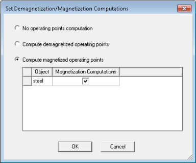
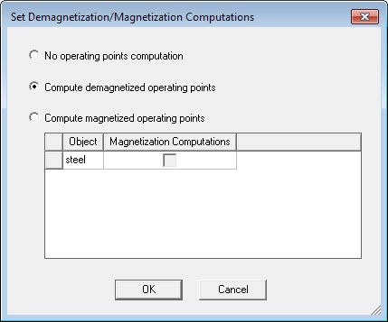
2. Click Maxwell > Excitations > Set Magnetization Computation to open the Set Demagnetization/Magnetization Computations dialog box.

   You can also open the Set Demagnetization/Magnetization Computations dialog box by right-clicking Excitations in the Project Manager, then selecting Set Magnetization Computation on the context menu; or by right-clicking in the Modeler window and selecting Assign Excitation > Set Magnetization Computation.

3. Select Compute magnetized operating points, and select the objects for magnetization and/or hysteresis-based magnetization computation, then click OK to accept the settings and close the dialog box.

   

4. Solve the design and the solution will include the element-based magnetization data, and/or hysteresis-based demagnetization curve if the design uses nonlinear materials with non-zero Hc defined.

Second Design: Set up a Demagnetization design with Output of the Hysteresis-Based Magnetization Computation

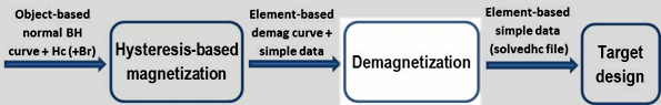
1. Create another Maxwell 2D or 3D magnetic transient design to be used as the Demagnetization design (highlighted above).
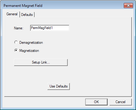
2. In the Project tree, right-click Excitations and select Assign > Permanent Magnet Field.

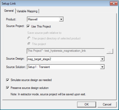
3. In the Permanent Magnet Field dialog box, select Magnetization, then click Setup Link.

   

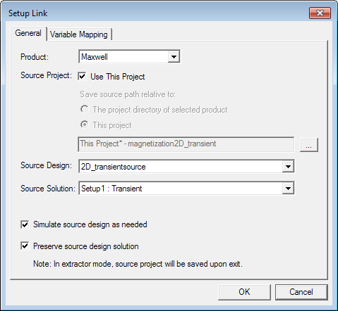
4. Set up a link to the Hysteresis-based magnetization computation source design (the first design you set up), which provides the hysteresis-based magnetization solution data. Check Simulate source design as needed and Preserve source design solution. If the source design is not set up to Compute magnetized operating points, an error message will be issued.

   

5. Right-click Excitations in the Project tree and select Set Magnetization Computation on the context menu to open the Set Demagnetization/Magnetization Computations dialog box, and select Compute demagnetized operating points.

   

   Note: Steps 6 and 7 are applicable only for object-based magnetization/demagnetization links. Omit these steps if design-based magnetization/demagnetization links are used.
6. Open the Solve Setup dialog and select Import mesh on the Advanced tab to open the Setup Link dialog box.
7. In the Setup Link dialog box, for the Source Design, choose the Hysteresis-based magnetization computation (the first design you set up).
8. Solve the design and the solution will include the element-based demagnetization distribution curve (which is based on the Hysteresis-based magnetization data). If the source design has not been solved, solving the current (demagnetization) design causes the source design to be solved first.

Third Design: Set up the Target Design

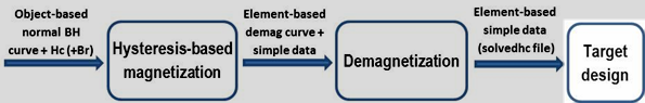
1. Create a third Maxwell 2D or 3D magnetic transient design to be used at the Target design (highlighted above).
2. In the Project Manager tree, right-click Excitations and select Assign > Permanent Magnet Field.

3. In the Permanent Magnet Field dialog box, select Demagnetization, then click Setup Link.

   

4. Set up a link to the Demagnetization design (the second design created above), which provides the dynamic demagnetization distribution solution data (based on the Hysteresis-based magnetization solution data from the first design). Be sure to check Simulate source design as needed and Preserve source design solution.

   

   Note: Steps 5 and 6 are applicable only for object-based magnetization/demagnetization links. Omit these steps if design-based magnetization/demagnetization links are used.
5. Open the Solve Setup dialog and select Import mesh on the Advanced tab to open the Setup Link dialog.
6. In the Setup Link dialog box, for the Source Design, choose the Demagnetization design (the second design created above).
7. Solve the Target design. If the source designs for hysteresis-based magnetization computation and demagnetization are not yet solved, solving the current (target) design causes the two source designs to be solved in sequence first.

Related Topics 

Setting Demagnetization/Magnetization Computations for Source Designs

Permanent Magnet Field Excitations for 2D and 3D Transient and Magnetostatic Solvers