
Specifying B-H Curves for Nonlinear Relative Permeability
For Maxwell 2D and 3D eddy current, magnetostatic, and transient solution types, when you define a new material or edit an existing material with a nonlinear relative permeability in the View/Edit Materials window, you need to specify the magnetization characteristics using B-H curves.
You can also model temperature dependencies of the nonlinear material property by providing two or more temperature-dependent B-H curves. For temperature dependencies of permanent magnetic materials, refer to Interpolation of Temperature-Dependent Demagnetization Curves.
If a user-input B-H curve is used without smoothing, the non-smoothed B-H curve is treated as piece-wise linear between user-input data points inside the software, which may cause nonlinear convergence issues. However, if you chose to use a smoothed B-H curve constructed by the software, the operating point may not exactly reside on the user-input B-H curve. Smooth B-H curve is not selected by default. You can select it from the Solve Setup, on the Solver panel. For isotropic nonlinear materials, you can force Maxwell to use the original user-input data points without smoothing by software by clearing the Smooth B-H Curve option.
- Open the View / Edit Materials
dialog from the Edit Materials window either by:
- Selecting an existing material that you need to edit, and click View / Edit Material.
- Clicking Add Material.
Either of these actions open the View/ Edit Materials window.
- For the Relative Permeability property,
do one of the following (depending on the type of material you are defining):
- Select Nonlinear as the Type. A B-H Curve button appears in the Value column.
- Select Anisotropic as the Type to display the additional parameters: T(1,1), T(2,2), T(3,3). Selecting Nonlinear for any of these additional parameters also causes a B-H Curve button to appear in the Value columns.
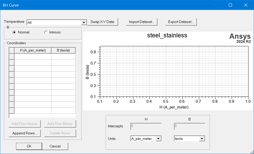
- To input B-H curve(s), click the B-H Curve button to open the BH Curve
window:
- A normal B-H curve is defined in the first quadrant and starts from the origin (0, 0). Here, “normal” means the curve starts from (0,0), instead of a curve type of Normal or Intrinsic.
- A demagnetization curve is defined in the second quadrant and may extend to the first and/or third quadrants, in which the first and last points are not oddly symmetric.
- A hysteresis curve is a branch of a major hysteresis loop: the ascending or descending branch. The ascending branch is defined through the third, fourth, and first quadrants, and the descending branch is defined through the third, second, and first quadrants. For either branch, the first and last points must be oddly symmetric.
- Set the Units for H and B by selecting from the drop-down menus. If temperature-dependent B-H curves are used, the selection of units is applied to all of the temperature-dependent curves.
- Choose the type of curve you want to define
by selecting either Normal or Intrinsic.
For a material property without an existing B-H curve definition, the default type will be Normal. For a property with existing B-H curve definition, the selected radio button corresponds to the existing B type.
Note:- The Intrinsic B-H curve is supported only in Maxwell 2D/3D magnetostatic, eddy current, and transient design types. A material property defined using an Intrinsic B-H curve will fail validation check in all the other product/design types.
- When an Intrinsic B-H curve is added, the Relative Permeability Value button label in the View/Edit Material dialog box changes to Bi-H Curve as visual indication of the type of curve currently defined for the material.
You can change the type at any time. For an existing curve, validation checks are performed on the coordinate list when you attempt to change the type. If the data is not valid, an error message will be displayed and the type of B will not be changed. If data is valid, a query dialog box displays asking if the coordinates should be converted.
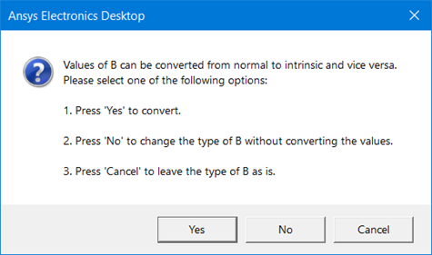
Click No if you have specified the B-H coordinates and then realize that you haven't select the desired type.
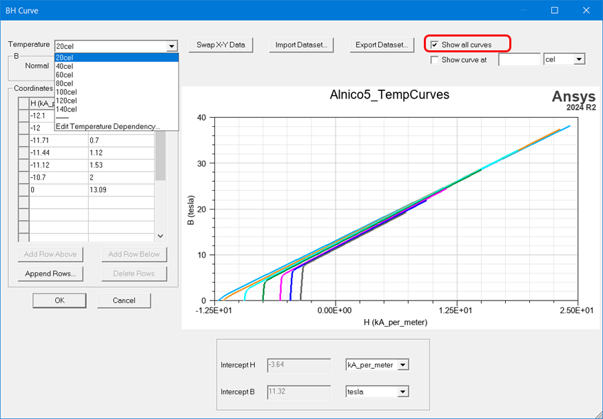
Note: Changing the type of the B-H curve invalidates all solution data. - The initial selections in the Temperature drop-down menu include All and Edit Temperature Dependency….
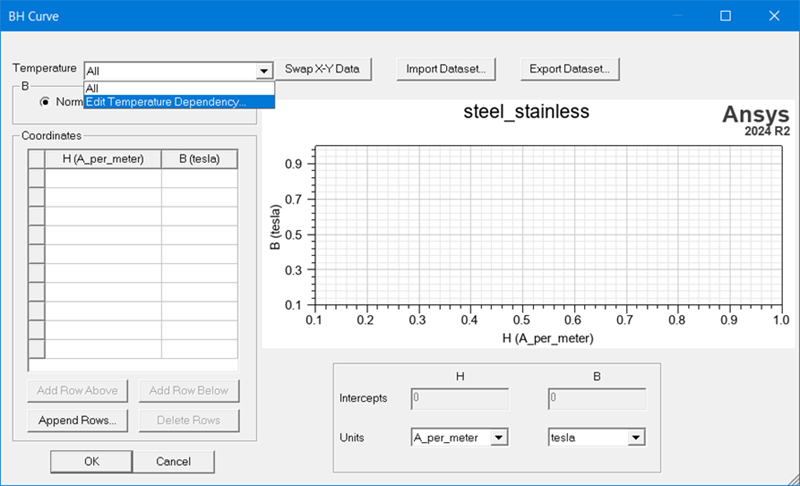
The default selection is All, which means the B-H curve applies to all temperatures – in other words, the B-H curve is not temperature-dependent. To define B-H curves with temperature dependency, see step 9.
- Enter B and H values in each row of the
Coordinates table. Placing the
cursor in a table cell enables the Add Row
Above, Add Row Below,
and Delete Rows buttons.
Append Rows allows you to specify the number of rows
to append to the table.Note:
- When using temperature-dependent B-H curves, the settings in the B-H Curve dialog apply to the currently selected temperature value.
- When adding (or editing) temperature-dependent B-H curves, repeat this step for each specified temperature as needed.
Note the following requirements for creating a valid curve:
- For a Normal B-H curve, the slope of the curve can not be less than that of free space anywhere along the curve.
- For an Intrinsic B-H curve, the slope of the curve can not be less than 0.
- The value of B must increase along the curve.
- The initial value of B must be 0 (zero).
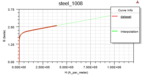
- Because B-H operating points in the FEA solution may extend beyond the input B-H data set, the B-H data set is extrapolated in Maxwell. The slope of the last two user-defined data points is used to extrapolate the B-H curve, and thus should be as close to μ0 as possible.
- The data points representing the B-H curve should have enough points for accurate representation of the curve. Twenty (20) or more points should be specified with increased representation on the "knee" of the curve.
- Normal B-H curves with a positive B value at
the first point will be extrapolated (interpolation). Intrinsic curves are not extrapolated.
As you enter values, the graph is updated. If you are using multiple temperature-dependent B-H curves, a Show all curves check box is present. Checking this box enables all of the temperature-dependent B-H curves to be displayed simultaneously.
- Optionally, click Import Dataset to import
B-H curve data from a file, and if they are in the wrong columns, click
Swap X-Y Data to switch the B
values and H values in the graphics display. You can also use the SheetScan
tool to extract curve data from sources such as manufacturer datasheets
to a dataset, which can then be exported to a tab-delimited file, and
imported via Import Dataset. (Refer
to Adding Datasets and Exporting Datasets for related information
on working with datasets. Refer to Using SheetScan for working with the SheetScan
tool.)Note: When using temperature-dependent B-H curves, selecting Import Dataset will import a single curve for the currently selected temperature.
-
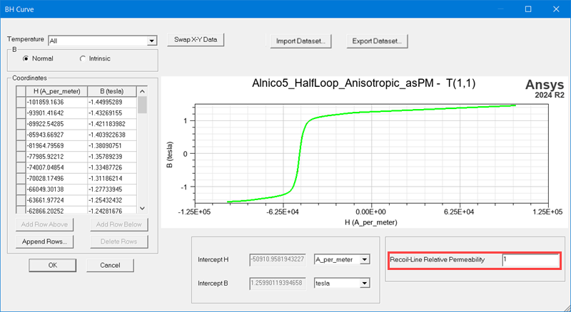
For a hysteresis curve only, set the Recoil-Line Relative Permeability. When a magnetic field is fully saturated, a (B, H) operation point will trace the major hysteresis loop, which consists of an ascending curve and a descending curve. The operation point will trace a recoil line when B or H reverses its direction locally, as shown in the following figure. For most hysteresis materials, the recoil-line relative permeability is 1.0. When you input a hysteresis curve, you need to ensure that the slope between any two adjacent points are not smaller than the recoil-line slope.
- Optionally, for Maxwell 2D and 3D eddy current, magnetostatic and transient solution types, you can model temperature dependencies of the nonlinear material property by providing multiple temperature-dependent B-H curves. At least two B-H curves must be defined when using this feature. If you want to change the Temperature setting to specify temperature-dependent B-H curves:
- Select Edit Temperature Dependency to open the Edit Temperature Dependency dialog box.
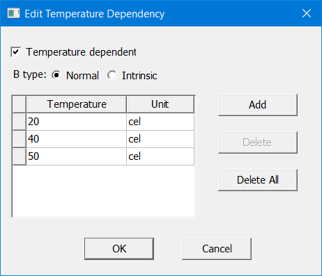
- Use the Add button to add rows to the table. In each row, enter the desired Temperature, and select the appropriate Unit. The Delete button can be used to remove selected rows from the table. Delete All removes all of the rows.
- Check Temperature dependent to enable temperature-dependent BH curves to be added.
- Click OK to return to the BH Curve dialog box.
The Temperature drop-down menu now lists all of the temperatures you specified above. Select the one for which you want to enter B and H coordinate values in the following step. Also, a Show all curves check box is now present. Checking this enables all of the B-H curves to be displayed simultaneously.
The Show curve at option can be used to show the interpolated curve for a temperature value not specified in the B-H data.
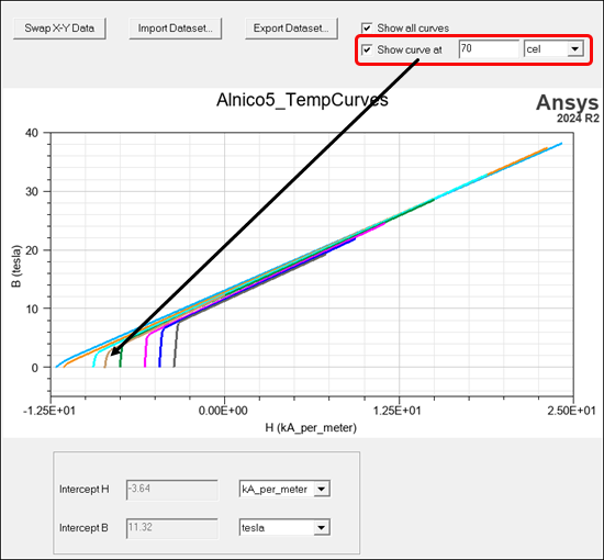 Note: The Show curve at option only works for demagnetized curves that have Intercept H and B starting at non-zero values.
 - Select Edit Temperature Dependency to open the Edit Temperature Dependency dialog box.
-
When finished entering data, click OK to close the window.
An error message displays if a slope is out of tolerance, identifying the data points between which the slope is less than that of free space. Out of tolerance data points must be corrected before you can successfully exit the dialog box. If the slope of the last two points is more than twice the permeability of free space, a warning message is issued during the solution. The slope of the last two points should be as close to μ0 as possible to represent a fully saturated material.
You can define one of the following three kinds of B-H curves: normal B-H curve, demagnetization curve, or hysteresis curve:

The B-H curve (or curves if multiple temperature dependencies are used) you have defined is associated with the Relative Permeability property of the material.