Setting HPC and Analysis Options for Maxwell and RMxprt Designs

All analysis configurations are accessed via a single window. The machine list and options settings have been integrated into analysis configurations. The default configuration is for solving on a single, local machine. You can create many analysis configurations for remote and distributed solutions and switch between them depending on the job being solved. Multiprocessing has been integrated into the machine lists.

To set HPC and Analysis Options:

Click Tools > Options > HPC and Analysis Options.
You can also access HPC and Analysis Options using the HPC Options icon on the Simulation ribbon.
The HPC and Analysis Options window appears, displaying the Configurations tab.

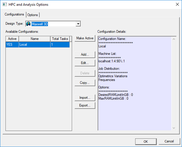
Configurations Tab

Available Configurations are described by Name, whether or not they are Active, and the Total Tasks the configuration can execute. Selecting a configuration from the list displays the details of that configuration in the Configuration Details panel.

From the Configurations tab, select the Design Type to display a list of available configurations for that type.

Configurations can be created for each design type. To use similar analysis parameters for different design types, create separate analysis configurations for each design type. The active configuration is used when solving an analysis for that design type.

Assigning a Design Type to a configuration

Selecting an Available Configuration

To activate a configuration, select it from the Available Configurations list and click Make Active. The active configuration will be indicated by a YES in the Active column.

Additional options include

Add – launches a window to create a new analysis configuration.
Edit – launches a window to edit the currently selected analysis configuration.
Delete – deletes the currently selected analysis configuration(s).
Note: You cannot delete the Local configuration.
Copy – creates a new analysis configuration, and launches a window to edit it. If the window is canceled, the new analysis configuration is not created.
Import – allows you to import an *.acf file to create an analysis configuration.
Note: Importing analysis configurations always adds the imported analysis configurations to the current design type. If there is a name conflict between an imported analysis configuration and an existing analysis configuration, the imported configuration is renamed and a notification appears.
Export – allows you to export the selected analysis configurations to an *.acf file. You can then import the configurations into a different design type, or import them on a different machine.

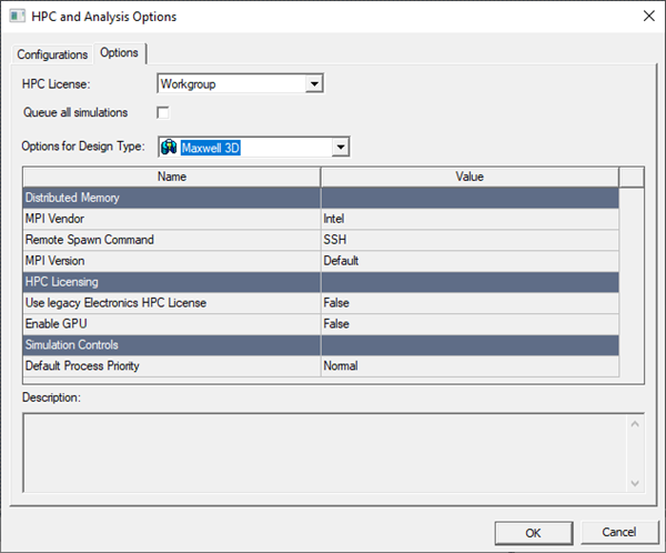
Options Tab

The Options tab in the HPC and Analysis Options window contains general and product-specific settings:

HPC and Analysis Options window's Options tab

Important: Available options vary by design type. Certain items discussed on this page may not be visible, depending on the currently selected design type.

These options are not specified for or saved as part of the current analysis configuration. Instead, they are global and are always in effect for the given design type when both of the following conditions are true:

A design of the matching design type is being solved.
You have not specified corresponding overriding batch options on the command line.

From the Options tab, you can

choose the HPC license type
enable queuing
specify Distributed Memory settings (for example, MPI for certain solvers)
set licensing options
enable GPU (for Transient, Matrix and SBR+ solves)
set the Default Process Priority

Note: Solving with Intel MPI on a single Windows machine does not require MPI installation, but registration of the user's password with Intel MPI on the host is required if using password authentication. Solving with Microsoft MPI on a single Windows machine requires Microsoft MPI to be installed and the MS-MPI Launch Service to be started. These steps are not required for Microsoft MPI analysis on a Windows HPC cluster. Solving with Microsoft MPI on multiple Windows hosts is only supported on a Windows HPC cluster.

Users running on Linux do not need to install MPI manually.

For HPC License, select Workgroup or Pack.

HPC licensing enables the use of cores and GPUs to accelerate simulations. In general, each core requires one unit of HPC, while each GPU requires eight units. The selected HPC license type determines which license is used and how units of HPC are converted to license counts.

Workgroup (formerly "pool") – One HPC workgroup license enables one unit of HPC.
Pack – One HPC pack license enables eight units of HPC. Additional packs multiply by four, enabling 32, 128, 512,... , in the context of a single simulation.

Electronics Desktop products include four units of HPC for each licensed simulation. This means that up to four units can be used without requiring HPC licenses; license counting begins with the fifth unit. For example, a simulation that uses 36 cores requires 32 HPC units after subtracting the four included cores. This simulation will check out 32 HPC workgroup licenses, or two HPC pack licenses.

HPC licenses enable all parallel and distributed simulations, including distributed variations. Distributed variations require a single set of solver licenses, plus HPC to enable the variations.

For HPC Workgroup, distributing N variations requires 8*(N–1) workgroup licenses and, together with the solver licenses, enables up to four HPC units per variation. Each additional set of N workgroup licenses will enable one additional HPC unit per variation. For HPC Pack, distributing N variations requires N–1 pack licenses and, together with the solver licenses, enables up to four HPC units per variation. Each additional set of N pack licenses will enable 8, 32, 128,... additional HPC units per variation.

Ansys licensing supports distributed simulations when Electronics Desktop is called from other Ansys tools, such as optiSLang and Workbench. In such cases, distributed design points (variations) generally use HPC counts as described above.

Note: Licensing for some calling products may include some distributed design points, in which case the total required HPC will be reduced.

If the Queue all simulations check box is selected, the Desktop queues any active simulations for design types that have Save before solving turned off in the General Options and then processes them in order. You can view and change the queue by using Show Queued Simulations.

To configure options:

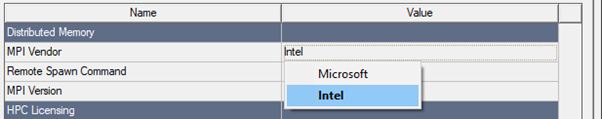
Under Distributed Memory, for solvers that use MPI (HFSS, HFSS 3D Layout, Icepack, Maxwell, and Q3D) use the drop-down menu to select the MPI Vendor for the selected design type:
The solvers use the industry-standard Message Passing Interface (MPI) and can perform solutions that distribute memory use across machines in a cluster or network. Memory used by the MPI-enabled solver is therefore limited by the set of machines that is available rather than the shared memory available on any single machine. This allows you to simulate larger structures and to optimally reconfigure the cluster of machines for the problem at hand. For solving on a single machine, MPI is not required nor does it provide an advantage.
To use the distributed memory solution, you need to install MPI software from a supported third-party vendor on all the machines you intend to use.
Depending on the MPI vendor, you may need to set passwords for authentication on the machines. Settings within each design type turn on distributed memory solutions and define the list of machines you intend to use.
Specify the MPI version. If not specified, the default version for the MPI vendor will be used. This setting is ignored if there is only one supported version for the selected MPI Vendor. Multiple versions are only supported for Intel MPI, as follows:
- The value Default indicates that the default Intel MPI version should be used. This is Intel MPI 2018 in most cases.
- The value 2018 indicates that Intel MPI 2018 should be used.
- The value 2021 indicates that Intel MPI 2021 should be used.
By default, MPI vendors use the fastest interconnect by default (for example, InfiniBand is typically faster than Ethernet). If you want to override the default behavior and force the use of Ethernet, you can set the ANSOFT_MPI_INTERCONNECT environment variable to "eth" for the job.

For Linux authentication, specify the Remote Spawn command as RSH or SSH (the default).
Electronics Desktop supports GPU acceleration for transient, frequency domain, SBR+, and Maxwell 3D eddy current matrix solutions.

Optionally, you can select one of the following from the Default Process Priority drop-down menu:
- Critical (highest) (Not recommended)
- Above Normal (Not recommended)
- Normal (Default)
- Below Normal
- Idle (lowest)

You can also set these values using VB or Python scripts.