Magnetostriction Modeling of Magnetic Material
Magnetostriction was first observed by J. Joule in 1842. Currently, it is typically described as "deformation of a body" as a result of its magnetization. The elongation or contraction in the direction of applied magnetic field is usually between 10-5 and 10-3 and accompanied by the opposite sign changing in the transverse direction, so that the volume remains almost the same. The phenomenon of magnetostriction can be regarded as an energy transduction (or transformation) from mechanical to magnetic and vice-versa. It can be described as a bidirectional magneto-mechanical coupling between the mechanical and magnetic fields in the magnetostrictive material. The origin of this phenomenon can be traced to the alignment of the magnetic domains inside the material. The following figure is a schematic of the effect simplified to one dimension.
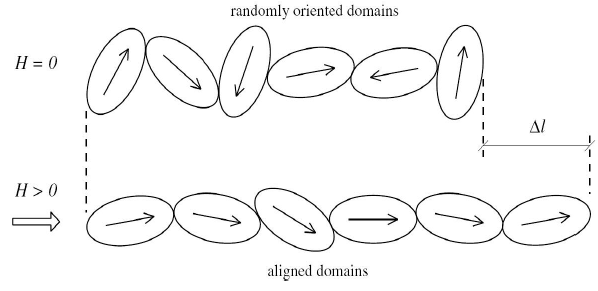
When no magnetic field is applied to the system, the series of domains have randomly oriented magnetic moments. Whereas when a magnetic field is applied, the series of domains rotate to partially align themselves to the magnetic field direction, resulting in a change in length ∆l. Applying a sufficiently high magnetic field will result in perfectly aligned domains, in which case the material achieves the maximum magnetically induced strain (that is, peak magnetostriction). Magnetostriction requires the magnetic domains to be longer in one dimension than the other two to obtain a change in length when the domain rotates. This, in general, results in anisotropy of the crystal structure of the material.
Magnetostriction is considered to be one of the main sources of noise in transformers. When an alternating voltage is applied to one or more windings of a transformer, a magnetic flux is generated in the transformer core laminations made of grain-oriented electrical steel. The nonlinear anisotropic property of magnetostriction creates alternating changes of the core dimensions due to the varying magnetic flux in the laminations. Those magnetostrictive forces cause core vibrations that are transmitted to the tank via the insulation oil and the core clamping points. Part of the mechanical energy is eventually radiated by the tank walls as noise. In electric motors, magnetostrictive forces also contribute to motor vibration and noise.
On the other hand, magnetostrictive materials convert energy between the mechanical and magnetic domains (inverse magnetostriction). They deform in response to applied magnetic fields and change their magnetic state when stressed. Some materials (such as Terfenol-D, Galfenol) have the ability to produce large magnetostrictive strains at moderate fields. Short response times (in the millisecond range) combined with resolutions in the order of microstrains make these materials well-suited to precision sensing and actuation mechanisms.
Due to the complexity of the mechanism of magnetostriction, it is very difficult to predict it with analytic models. In general, empirical methods based on statistics and dimensional basic parameters are used by most transformer manufacturers and sensor producers. Those approaches present limitations when applied to new designs and do not enable accurate parametric studies. Therefore, prediction models based on finite element formulations will be utilized to accurately describe the complex interactions of the various design parameters and the coupling of the physical fields.
The finite element method (FEM) is widely used in engineering practice because using the irregular grids, it can model complex inhomogeneous and anisotropic materials and represent complicated geometry. The FEM discretization produces a set of matrix differential equations. Because of the nonlinearity, the matrices generally are dependent of the solution vectors, so an iteration method such as Newton-Raphson method should be used to solve these nonlinear matrix equations. Namely, the nonlinear matrix equations are linearized for each nonlinear iteration. The linearized matrix equations may be solved by either a direct or iterative matrix solver.
The governing equation of magnetic field is given by

|
(Equation 1) |
Where A is the magnetic vector potential, σ is the electrical conductivity, and µ is the magnetic permeability of material. J represents the current density.
The magnetic flux density B can be expressed as:
| B = Ñ x A | (Equation 2) |
The relationship between B and H (magnetic field) is based on the constitutive law:
| B = mH | (Equation 3) |
For a discretized mechanical system, the governing equilibrium equation can be written as
| Kr + R0 = R | (Equation 4) |
where K is the system stiffness matrix, R0 is the body force vector, and R the vector of external force, r is vector of node displacement. The strain-displacement relationship can be written as
| S = Ñr | (Equation 5) |
Where S is the strain tensor. And the stress-strain relationship can be described by
| T=CS | (Equation 6) |
where T is the stress tensor, and C is stiffness matrix.
When a magnetic field is applied to a magnetostrictive material, strain occurs within the material placed in a magnetic field in response to the flux density within the material, while the stress gives feedback to affect the magnetic field. For coupled method, we have
|
|
(Equation 7) |

|
|
(Equation 8) |

|
|
(Equation 9) |

Where d and dt are magneto-mechanical coupling coefficients, λ is magnetostriction induced by magnetic field H. The magnetic field and mechanical stress field are solved together, which means both fields are solved on the same mesh simultaneously by using the one matrix solver.
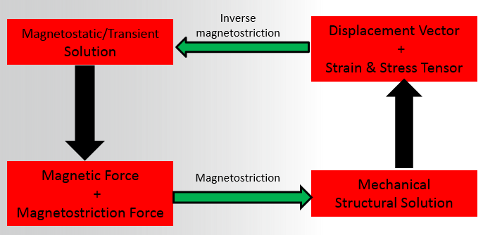
For decoupled method, the magnetostriction may be determined once the magnetic field distribution is obtained from FEM simulation. Hence, an elastic analysis is reduced to the problem of finding the stress due to an external load caused by a force applied to a material with a previously known magnetostriction, the latter unrelated to the stress. Magnetostriction is transformed into stress with the usage of Hooke’s law. Equation (7) can be rewritten as:
| B = mH + dT | (Equation 10) |
| S = C-1T + dTH | (Equation 11) |
where
dTH: magnetostrictive, deformation induced by magnetic field H.
dT: inverse magnetostriction, impact of stress T on magnetic field B.
By using the decoupled method, the magnetic field and stress field can be solved independently with different mesh and different solver, and magnetostriction and inverse magnetostriction can be involved in either one or both. Compared to the coupled method, the decoupled method is more flexible and general. The process for the decoupled method is shown in the following figure: