Frequency Domain (Eddy Current) T- W Solver

The 3D eddy current solver (frequency domain or harmonic solver) uses the formulation. It is based on the assumption that all electromagnetic fields pulsate with the same frequency (specified by the user) and have magnitudes and initial phase angles calculated by Maxwell. There are no moving objects (velocity is zero everywhere). Permanent magnets cannot be part of the model, and all materials are assumed to be linear theoretically.

For designs with nonlinear materials, analysis is based on the fundamental components of B and H at a specified frequency as an approximation. See Nonlinear Eddy Field Simulation for more information.

For nonlinear systems, the Eddy Current solver can be used as an alternative to the transient solver to solve for harmonic losses.

Electromagnetic radiation can also be simulated.

In the non-conducting regions the magnetic field strength is given by the following equation:

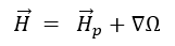
using node element with the same quadratic approximation as for the case of the magnetostatic solver.

In regions with non-zero conductivity where eddy current calculation has been set up, the following equation is true:

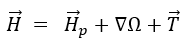
where is the electric vector potential calculated using edge elements. At the interface between conductors and non-conductors the tangential component of the electric vector potential is constrained to zero.

The default order of the magnetic scalar potential is 2, and the default order of the electric vector potential is 1.

The quantity calculated by Maxwell is in this case the magnetic field H(x,y,z).

For eddy current problems, typical sources associated with non-winding excitation are current and current density; typical sources associated with winding excitation are current and voltage. In applying the sources for the magnetic field problems, keep in mind that the applied current distribution must be divergence free in the entire space of the solution as it is physical for (quasi) stationary conduction current density distributions. Thus, the conduction paths(s) for the applied current distributions must be closed when totally contained within the solution space for the problem or must begin and end at the boundaries. The total current applied to conductors that touch the boundaries doesn't require the existence of terminals at the ends where the current is applied, the respective planar surfaces of the conductors in the plane of the region (background) can be used to apply the excitations.

Typical boundary conditions used in eddy current problems include magnetic field tangent (the default, natural boundary condition which is automatically applied on all surfaces of the problem space -the surfaces of the geometry entity containing the model inside it). This default boundary condition can be overwritten if other boundary conditions are applied on exterior surfaces of the solution space. The default boundary condition confines the magnetic field to the solution space and thus this boundary must be placed at some distance from the sources of the problem to avoid over-constraining the fields by placing the boundaries to close to the model objects. While it is difficult to provide "recipes" with general validity on the placement of the boundaries of problems, a good rule of thumb says that if a model can be imagined as being contained in a sphere of radius R, the boundaries can be placed at a 4-5 radii R from the imaginary center of the model.

The Zero Tangential H Field allows you to prescribe a normal (in average) magnetic field orientation on an arbitrary surface. This boundary condition does not require any further user input, that is, no value and coordinate system specification are necessary.

In the case of Tangential H Field boundary condition the values of two tangential complex components (real and imaginary) and a surface coordinate system have to be defined and subsequently used in the assignment process of this boundary condition. This boundary condition is restricted to two kinds of surfaces: planar or cylindrical. The CS in the planar case would be a rectangular coordinate system with X and Y components of H in the plane. The coordinate system in the cylindrical case would be a coordinate system with a Z axis coinciding with the axis of the cylinder and the two components to input would be the PHI and Z axis components of H.

In the case of the tangential H field caution is advised: this boundary condition should be specified such that Ampere's theorem is not violated inside the field domain or at the boundaries. This boundary condition is very useful to simulate the behavior of devices "immersed" in an electromagnetic filed of desired magnitude and orientation.

Symmetry boundary conditions are used to solve problems with symmetry and thus allows the users to take advantage of the significant reduction of the problem size for a given accuracy. Symmetry boundary conditions are of two kinds, Odd (flux tangent) or Even (Flux normal). Although the use of this symmetry boundary condition overlaps with previous conditions to some extent, the symmetry boundary conditions should only be used in clear symmetry cases.

The Insulating boundary condition is of particular use for applications where very thin insulating layers are impractical to model due for example to high aspect ratio geometries that would be generated and associated meshing difficulties. Thus insulating boundary condition can be assigned to surfaces of separation between conductors. Another remarkable situation where such a boundary condition proves to be extremely useful is in modeling faults in conductors (cracks for example). Thus, modeling 2D (sheet) objects at the location of the respective cracks and applying the insulation boundary condition proves to be a very effective way of modeling the flaws without having to generate 3D cracks that would be difficult and impractical to mesh.

For more information on eddy current simulation setup, see Eddy Current Solver Settings