Coupling Maxwell Designs with Ansys Thermal via Workbench

Coupling Maxwell 2D/3D with Ansys applications is supported via the Workbench schematic. Thermal feedback is supported for Maxwell magnetostatic, eddy current, AC and DC conduction, and transient types. Users also need to set up the design and geometry appropriately. An appropriate design should be temperature-dependent, and have one or more solve setups that are enabled for thermal feedback.

1. The easiest way to add a Maxwell 2D or 3D design to a Workbench schematic is to import a working design via Workbench File > Import. The imported design is placed in the Workbench schematic after it is successfully imported.
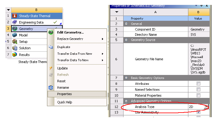
2. Next, insert a Steady-State Thermal system and change its Analysis Type to 2D or 3D, (depending on the Maxwell design type) by right-clicking on the Geometry cell and selecting Properties. It is important to change the Steady-State Thermal system's analysis type before setting up its geometry.



3. To set up the Steady-State Thermal system's geometry, you must first export the Maxwell geometry using sat or step format as follows:
1. Select the Modeler > Export menu item.
2. Select the desired model geometry format (sat or step), and the save location in the dialog box and save the file for use by Ansys Workbench.
4. Import the file via the Geometry module of the Steady-State Thermal system.
1. To access the Geometry module, double-click on the Geometry cell in the Steady-State Thermal system to launch Design Modeler.
2. Select File > Import External Geometry File and browse for the geometry file exported from Maxwell.
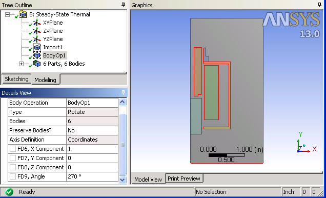
3. After the geometry file is imported, right-click on the root folder of the modeler project tree and select Generate. (When the geometry file is of a Maxwell 2D RZ design, users can rotate the geometry in Design Modeler by creating a body operation.)

   

5. Close Design Modeler and refresh the Model cell of the Steady-State Thermal system by right-clicking the Model cell and selecting Refresh.
6. The geometry mode of the Steady-State Thermal system can be changed via the Ansys Mechanical user interface.
1. Launch Mechanical by double-clicking the Setup cell of the Steady-State Thermal system.
2. Select Geometry in the project tree and the Definition of Geometry will be shown in the Detail window.
3. Select either Plane Stress or Axisymmetric as the value for the property 2D (or 3D) Behavior.
7. To set up the coupling, drag the Solution cell of the Maxwell system and drop it on the Setup cell of the Steady-State Thermal system.

   

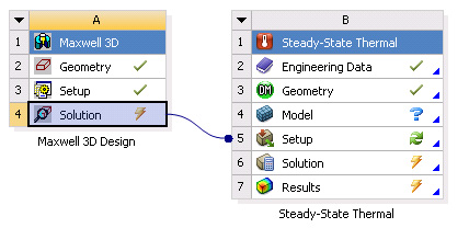
8. Note that the Maxwell Solution cell is tagged with a “Lighting Bolt” symbol. Right-click on the Maxwell Solution cell and select Update. This will initiate a Maxwell simulation if it is not already solved. Once Maxwell's solution is available, the “Lighting Bolt” changes to a “Green Check” symbol.
9. To “push” the coupling into Steady-State Thermal, right-click on the Steady-State Thermal Setup cell and select Refresh.
10. After refresh is finished, you can launch Ansys Mechanical by double-clicking the Setup cell to finish the coupling setup.
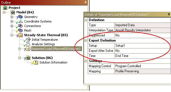
11. In the Ansys Mechanical application project tree, an Imported Load (Maxwell2DSolution) or (Maxwell3DSolution) item should already be inserted. Select the Imported Load folder to view its details. Because the inserted Maxwell 2D (or 3D) system supports thermal feedback, the Details window shows information regarding how the temperature result should be exported, and what type of mesh mapping should be used.

    

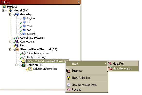
12. To finish the coupling setup, you must insert either an imported Heat Generation or an imported Heat Flux boundary condition. Heat Generation is used when mapping loss from objects in Maxwell; and Heat Flux should be used to map the loss from the edges of objects in Maxwell. Users can insert multiple Heat Generation or Heat Flux loads via the Imported Load (Maxwell2DSolution), or Imported Load(Maxwell3DSolution) objects.
Note: When setting up loss transfers from Maxwell to any other product within the WorkBench framework, if the user wants to map loss density on a face shared by two objects, this face only has to be used once in the setup.

13. To insert a Heat Generation, use Body select by clicking the icon in the Mechanical Toolbar. Then click on the objects where the EM loss should be imported. After all the desired objects are selected, right-click on Imported Load (Maxwell2DSolution) > Insert > Heat Generation, or Imported Load (Maxwell3DSolution) > Insert > Heat Generation.

    

A sub-item named Imported Heat Generation will appear in the project tree.

14. Click on the Imported Heat Generation tree item to view its details.

    

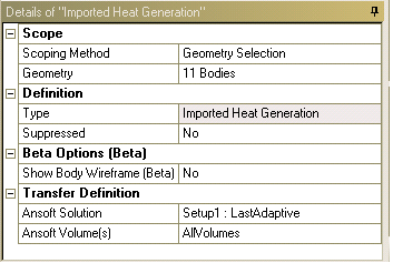
15. In the Transfer Definition section, users can set up the source Maxwell solution by pulling down the Ansoft Solution combo box and select one of the listed Maxwell solutions.
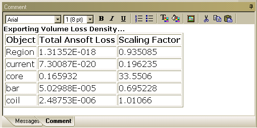
16. Right-clicking on Imported Heat Generation > Import Load will import loss from the Ansoft Solution selected for this load. After import has completed, the Import Heat Generation item becomes a folder, and an entry called Imported Load Transfer Summary is listed. Select the Imported Load Transfer Summary entry and the scaling factors used to export the load from Maxwell will be displayed in the Comment window.

    

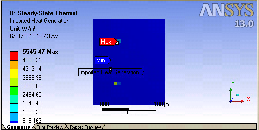
17. Selecting Import Heat Generation should show an overlay-plot of the imported load. The loss mapping from Maxwell can be verified by comparing this overlay-plot with an Ohmic-Loss field overlay plot in Maxwell.

    

18. Create a Convection boundary to complete the thermal setup:
    1. Use Edge select by clicking the icon at the Mechanical Toolbar and then Edit > Select All.
    2. With the edges selected, right-click on the Steady-State Thermal project tree item and insert a Convection.
    3. With the Convection item selected, change its Film Coefficient to 5 W/m2 via the Detail window.
    4. Right-click on the Solution tree item and select Solve.
    5. After the thermal solution is finished, insert a Temperature plot by right-clicking on Solution and selecting Insert > Thermal > Temperature.
    6. Right-click on the newly inserted Temperature item and select Evaluate All Results.
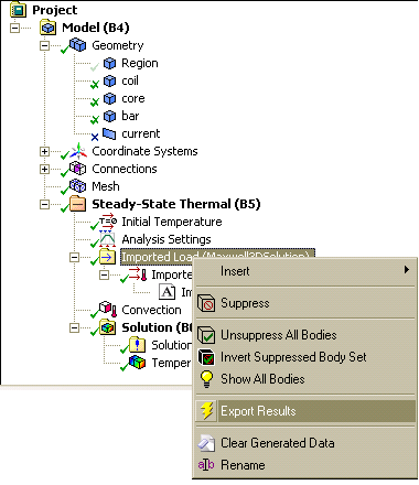
19. To export the thermal result to Maxwell, right-click on the Imported Load (Maxwell2DSolution), or Imported Load(Maxwell3DSolution) and select Export Results.

    

20. To fully utilize the automation capabilities provided in Ansys Workbench, select Imported Load (Maxwell2DSolution), or Imported Load(Maxwell3DSolution); and in its Detail window, select Yes for Export after Solve. With this option selected, users can continue the iteration between Maxwell/Thermal simulations from the Workbench schematic.

To “push” the exported thermal results back to Maxwell, right-click on Maxwell's Solution cell on the Workbench schematic and select Enable Update. Then, right-click again on Maxwell's Solution cell and select Update. This will trigger Maxwell to re-simulate its solution with thermal results.

To continue the solve iterations, repeat the following steps as needed:

1. Right-click on Thermal's Setup cell and select Refresh.
2. Right-click on Thermal's Setup cell and select Update.
3. Right-click on Maxwell's Solution cell and select Enable Update.
4. Right-click on Maxwell's Solution cell and select Update.

Related Topics 

Coupling Maxwell with Both Ansys Thermal and Structural via Workbench