
Assigning a Resistive Sheet Boundary for the 3D Magnetostatic Solver
For eddy current designs, refer to Assigning a Resistive Sheet Boundary for the Eddy Current Solver.
The Maxwell 3D magnetostatic solution can include a nonlinear resistive sheet boundary condition. The linear resistive sheet boundary condition is equivalent to a resistive sheet in the eddy solver and the transient solver (see links above). The nonlinear relationship between conductivity σ and current density J is as follows:

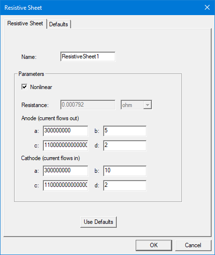
where L is the resistive sheet thickness, and a, b, c, and d are constants. For electric arc simulation, the nonlinear relationship is applied to both anode and cathode , so a total of eight constants are required – four for the anode and four for the cathode.
The ohmic loss on the nonlinear resistive sheet can be calculated using

where V is the resistive sheet volume, S is the resistive sheet surface, and

To define a resistive sheet boundary:
-
Select the section of the geometry on which you want to apply the boundary condition (typically a sheet object or face of a 3D conducting body touching another conducting body or face of a 3D conducting body touching the Region).
Note:- The sheet must be completely inside a conductor or on its surface.
- The sheet must have conductors touching both of its faces.
- The resistance value cannot be dependent on an intrinsic variable.
- Click Maxwell 3D > Boundaries > Assign > Resistive Sheet to open the Resistive Sheet dialog box. Alternatively, you can select the sheet/surface, right-click, select Assign Boundary > Resistive Sheet.
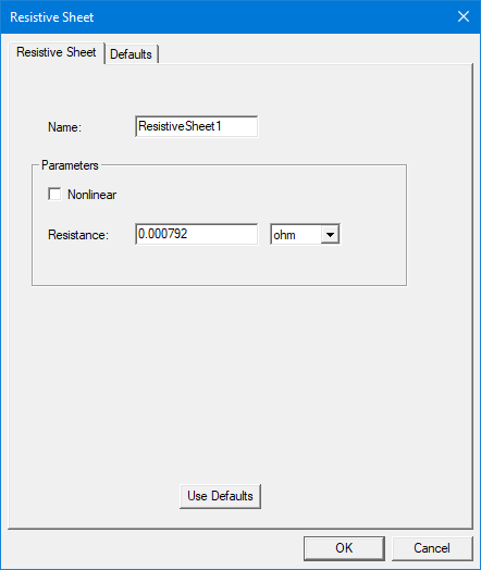
- Enter a name for the boundary in the Name box, or accept the default.
-
If Nonlinear is unchecked, enter a constant resistance value in the Resistance field, and select a unit of measure. Use of variables is supported. Constant resistance cannot be a negative value.
-
If Nonlinear is checked, additional fields display for entering Anode and Cathode values. These values correspond to the a, b, c, and d coefficients in the equations above. The a and b values cannot both be 0.
- Optionally, click Use
Defaults to revert to the default value (1 ohm) in the window.
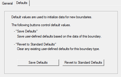
The Defaults tab allows you to control default values. The Save Defaults button saves the values currently defined on the General tab as the defaults to be assigned to new impedance boundaries. Revert to Standard Defaults clears existing user-defined values and replaces them with the standard default values.
-
Click OK to assign the boundary to the selected object.
The Project Manager lists the newly assigned resistive sheet boundary in the tree. You can select the boundary in the tree to view and edit its properties in the Properties Window. You can also double-click the boundary entry in the tree to open it for editing in the Resistive Sheet dialog box.
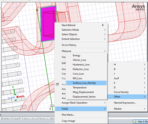
The losses incurred due to a Resistive Sheet boundary are output as Surface Loss Density. These losses are counted as losses in solid conductors and are reported together with the losses in other solid conductors under Solid Loss. If the Surface Loss Density is mapped to Mechanical, it should be assigned to a face as Heat Flux. The Surface Loss Density plot is accessed from Fields > Other.
Related Topics
Assigning a Resistive Sheet Boundary for the Transient Solver